9.3: Polar Coordinates and Functions
In Section 9.1 we introduced parametric equations and their utility to model various graphs. In this section we introduce a new coordinate system—polar coordinates—to further expand our scope of modeling curves. We discuss the following topics:
- Polar Coordinates
- Symmetry with Polar Functions
- The polar graphs of Circles, Lines, Spirals, Limacons and Cardioids, Roses, and Lemniscates
Polar Coordinates
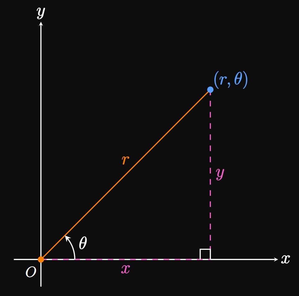
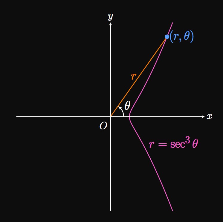
So far, we have used Cartesian coordinates (or rectangular coordinates), which represent a point in the \(xy\)-plane as \((x, y).\) We now use polar coordinates, which represent a point in a plane in terms of an angle \(\theta\) and distance \(\abs r\) from the origin. In Figure 1, a point in the plane is represented in polar coordinates as \((r, \theta).\) The angle \(\theta\) is formed between the positive \(x\)-axis—called the polar axis—and the line segment that connects the pole (denoted \(O\)) to point \((r, \theta).\) The angle \(\theta\) is positive if it extends in the counterclockwise direction and negative if it extends in the clockwise direction.
From Figure 1, we see \begin{equation} x = r \cos \theta \lspace y = r \sin \theta \pd \label{eq:polar-x-y} \end{equation} Moreover, \(\tan \theta = y/x\) and \(r^2 = x^2 + y^2.\) These formulas allow us to convert from polar coordinates to Cartesian coordinates, and vice versa.
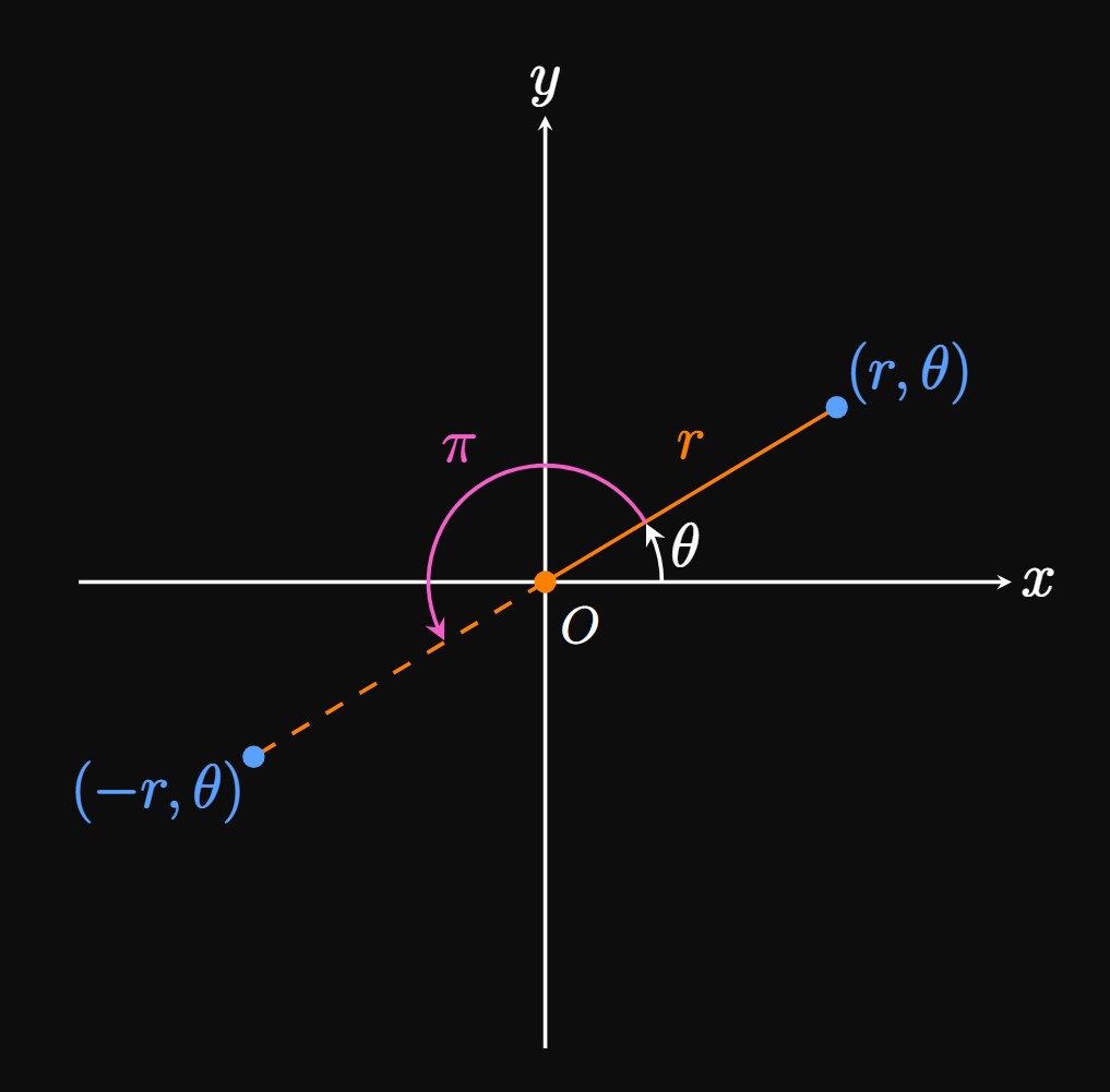
If \(r\) is replaced by \(-r,\) then the line segment that connects \(O\) to \((r, \theta)\) is rotated \(\pi\) radians about the origin, as in Figure 2. We write this new point either as \((-r, \theta)\) or \((r, \theta + \pi).\)
- \((4, \, \pi/4)\)
- \((7, \, 5\pi/6)\)
- \((-7, \, 5\pi/6)\)
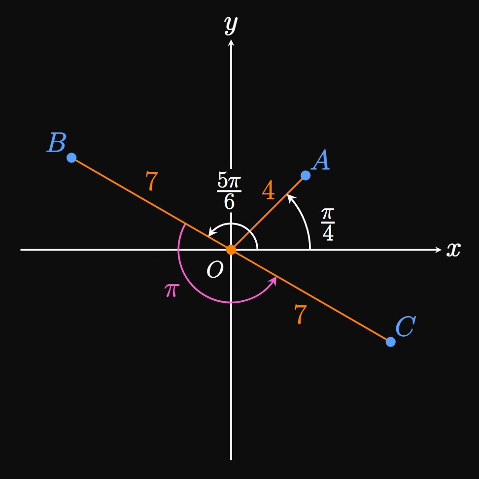
- We draw an angle that begins at the positive \(x\)-axis—the polar axis—and extends \(\pi/4\) radian in the counterclockwise direction. Then we draw a line segment that begins at the pole \((O)\) and extends \(4\) units. This point is labeled \(A\) in Figure 3.
- From the positive \(x\)-axis, we draw an angle that extends \(5 \pi/6\) radians in the counterclockwise direction. The line segment needs to extend \(7\) units from the pole. This point is labeled \(B\) in Figure 3.
- We follow the same procedure in (ii) but rotate the line segment \(\pi\) radians about the pole because \(r \lt 0.\) Hence, we obtain point \(C.\)
A polar graph is a graph defined by a polar function, \(r = f(\theta).\) For an input \(\theta,\) the distance from the pole is \(r = f(\theta).\) Many curves are best defined using polar functions. In addition, \(\eqref{eq:polar-x-y}\) enables us to define a polar curve using parametric functions, in which the central angle \(\theta\) is the parameter. To convert a polar function to a Cartesian equation, we want to express \(r\) and \(\theta\) solely in terms of \(x\) and \(y.\) The steps of conversion are as follows.
- Apply \(\eqref{eq:polar-x-y}\) [\(x = r \cos \theta\) and \(y = r \sin \theta\)] to express trigonometric functions in terms of \(x\) and \(y.\)
- Use \(r^2 = x^2 + y^2\) to rewrite \(r\) in terms of \(x\) and \(y.\)
- Use \(\tan \theta = y/x\) to express any remaining terms of \(\theta\) in terms of \(x\) and \(y.\)
Conversely, to convert a Cartesian equation to polar, we employ a similar strategy—expressing all \(x\) and \(y\) in terms of \(r\) and \(\theta.\) The steps are as follows.
- Apply \(\eqref{eq:polar-x-y}\) [\(x = r \cos \theta\) and \(y = r \sin \theta\)] to express \(x\) and \(y\) in terms of \(r\) and \(\theta.\)
- Convert any remaining terms of \(x\) and \(y\) to \(r\) by using \(r^2 = x^2 + y^2\) and \(\tan \theta = y/x.\)
- Isolate \(r\) if possible.
Symmetry with Polar Functions
Understanding symmetry helps us sketch graphs of polar functions. Recall the following properties of symmetry:
- The points \((x, y)\) and \((x, -y)\) are symmetric about the \(x\)-axis.
- The points \((x, y)\) and \((-x, y)\) are symmetric about the \(y\)-axis.
- The points \((x, y)\) and \((-x, -y)\) are symmetric about the origin.
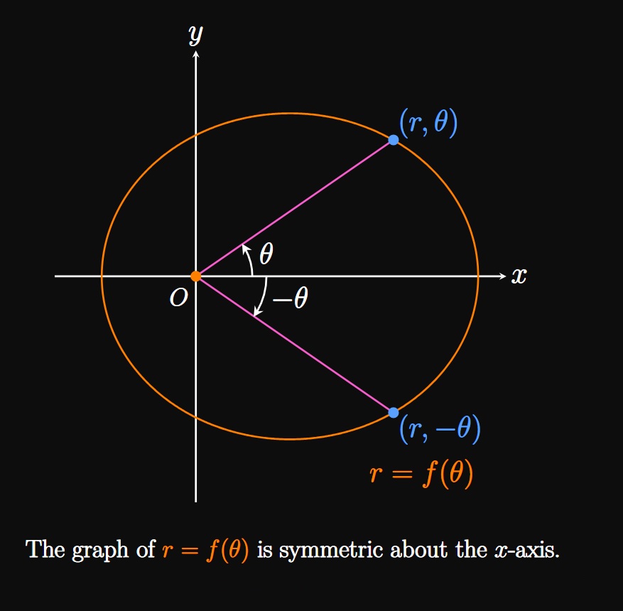
Because the angle
\(-\theta\) is a mirror of angle \(\theta\) across the \(x\)-axis,
the point \((r, -\theta)\) is a reflection of \((r, \theta)\) across the \(x\)-axis.
If a polar function \(f\) satisfies \(f(\theta) = f(-\theta),\)
then the graph of \(r = f(\theta)\) is said to be symmetric about the \(x\)-axis.
(See Figure 6A.)
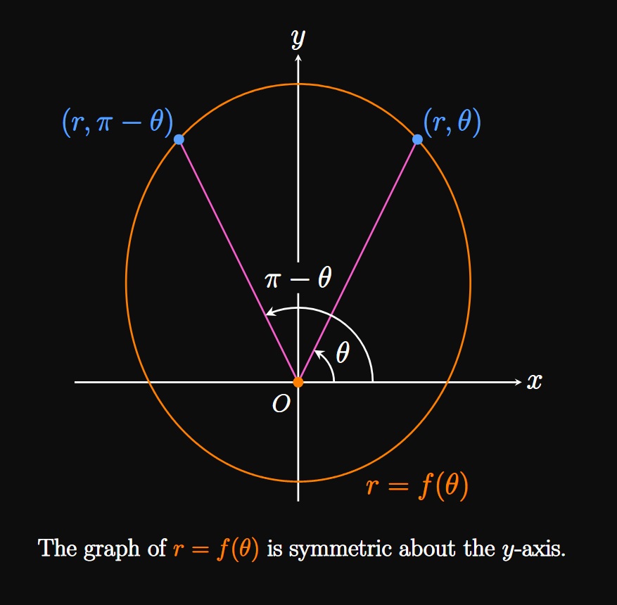
On the other hand, the point \((r, \pi - \theta)\) is a reflection of \((r, \theta)\) across the \(y\)-axis.
So if a polar function \(f\) satisfies \(f(\theta) = f(\pi - \theta),\)
then the graph of \(r = f(\theta)\) is said to be symmetric about the \(y\)-axis
(or about the ray \(\theta = \pi/2\)), as in Figure 6B.
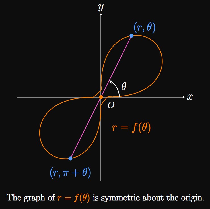
Lastly, rotating the point \((r, \theta)\) by \(180 \degree\) about the origin
gives \((r, \theta + \pi)\) or \((-r, \theta).\)
Hence, if the polar equation \(r = f(\theta)\) is unchanged if we replace \(r\) with \(-r\)
(or \(\theta\) with
- symmetric about the \(x\)-axis if \(f(\theta) = f(-\theta).\)
- symmetric about the \(y\)-axis if \(f(\theta) = f(\pi - \theta).\)
- symmetric about the origin if \(f(\theta) = -f(\theta + \pi).\)
Circles in Polar Form
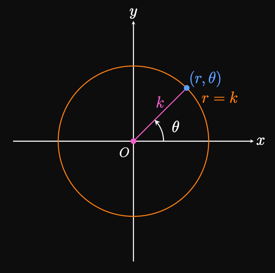
A simple polar graph is a circle of radius \(|k|\) centered at the origin. In Cartesian coordinates, this circle's equation is \(x^2 + y^2 = k^2.\) But we can convert this form to polar by using \(\eqref{eq:polar-x-y}\) [\(x = r \cos \theta\) and \(y = r \sin \theta\)]: Noting that \(\cos^2 \theta + \sin^2 \theta = 1,\) we obtain \begin{align} [r\cos \theta]^2 + [r \sin \theta]^2 &= k^2 \nonumber \nl r^2 (\cos^2 \theta + \sin^2 \theta) &= k^2 \nonumber \nl r &= |k| \pd \label{eq:polar-circle} \end{align} This equation is intuitive: at any value of \(\theta,\) the length of the line segment connecting the pole to a point on the circle is \(|k|.\) (See Figure 7.) Representing this circle is easier in polar form than in Cartesian form.
The key idea is to obtain values of \(r = 2 \cos \theta\) for some values of \(\theta,\) and plot and connect the corresponding points \((r, \theta).\) We assemble a table with convenient values of \(\theta,\) as follows.
| \(\theta\) | \(0\) | \(\ds \frac{\pi}{6}\) | \(\ds \frac{\pi}{4}\) | \(\ds \frac{\pi}{3}\) | \(\ds \frac{\pi}{2}\) | \(\ds \frac{2 \pi}{3}\) | \(\ds \frac{3 \pi}{4}\) | \(\ds \frac{5 \pi}{6}\) | \(\pi\) |
| \(r\) | \(2\) | \(\sqrt 3\) | \(\sqrt 2\) | \(1\) | \(0\) | \(-1\) | \(-\sqrt 2\) | \(-\sqrt 3\) | \(-2\) |
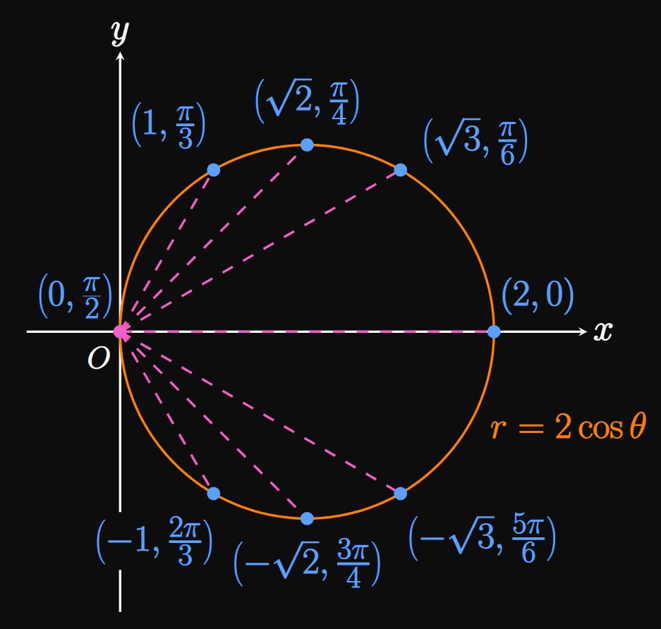
The standard form of a circle in Cartesian coordinates is \(\par{x - x_0}^2 + \par{y - y_0}^2 = k^2,\) where the circle is centered at \(\par{x_0, y_0}\) with a radius of \(k.\) We use the conversion formulas in \(\eqref{eq:polar-x-y}\) [\(x = r \cos \theta\) and \(y = r \sin \theta\)] and \(r = \sqrt{x^2 + y^2}\) to convert \(r = 2 \cos \theta\) into \begin{align} r &= 2 \, \frac{x}{r} \nonumber \nl r^2 &= 2x \nonumber \nl x^2 + y^2 &= 2x \nonumber \pd \end{align} We then complete the square to get \[x^2 - 2x + \orange{1} + y^2 = \orange 1 \implies \boxed{(x - 1)^2 + y^2 = 1} \] This circle is centered at \((x, y) =\) \((1, 0)\) with a radius of \(1.\)
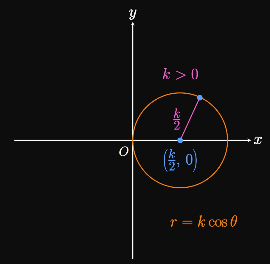
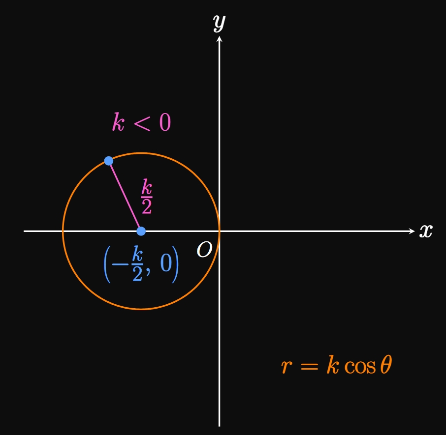
We now generalize Example 4 by considering the family of polar curves \(r = k \cos \theta.\) Replacing \(\cos \theta\) with \(x/r\) and \(r^2\) with \(x^2 + y^2\) gives \begin{align*} r &= k \, \frac{x}{r} \nl r^2 &= kx \nl x^2 + y^2 &= kx \pd \end{align*} We then complete the square to find \begin{align} x^2 - kx + \orange{\frac{k^2}{4}} + y^2 &= \orange{\frac{k^2}{4}} \nonumber \nl \par{x - \frac{k}{2}}^2 + y^2 &= \frac{k^2}{4} \pd \label{eq:polar-kcostheta} \end{align} Hence, the graph of the polar function \(r = k \cos \theta\) is a circle centered at \((x, y) = \par{k/2, \, 0}\) with a radius of \(|k/2|.\) By \(\eqref{eq:polar-kcostheta},\) if \(k \gt 0,\) then the circle is centered on the positive \(x\)-axis (Figure 9A). Likewise, if \(k \lt 0,\) then the circle is centered on the negative \(x\)-axis (Figure 9B).
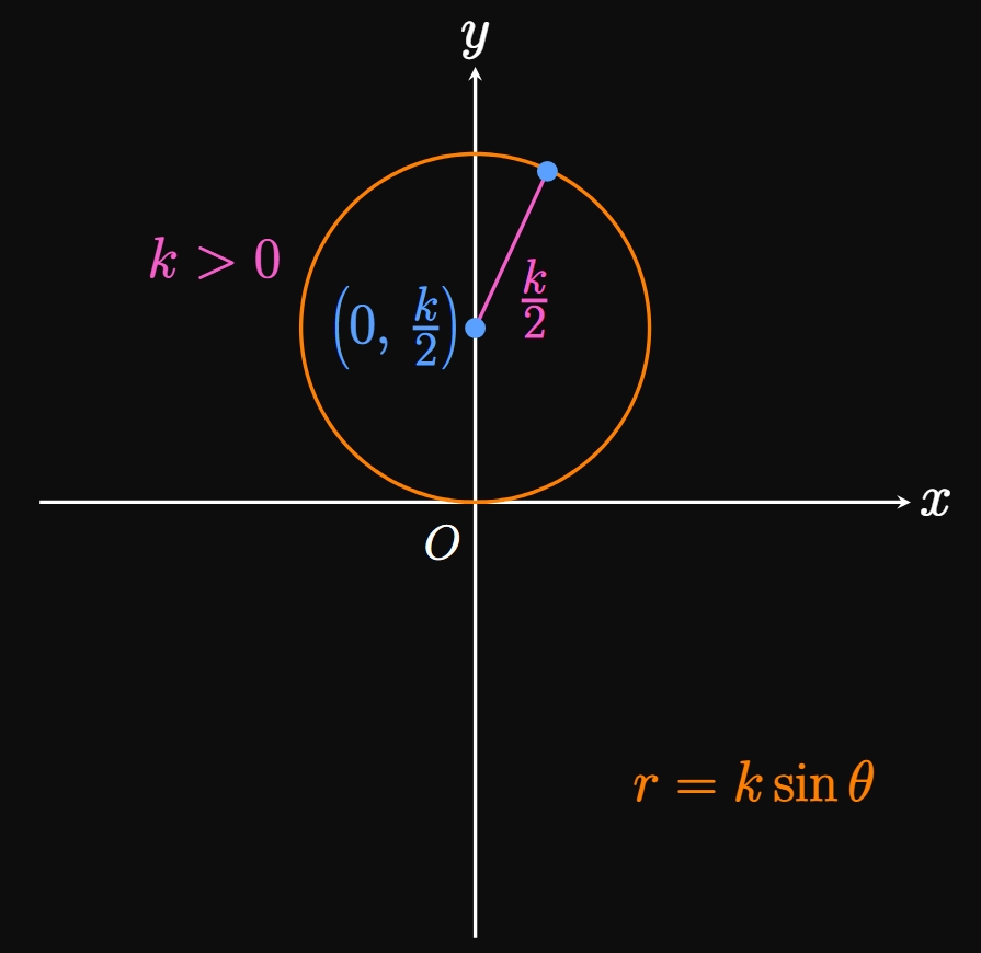
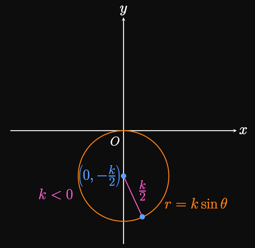
Likewise, we can convert \(r = k \sin \theta\) to a Cartesian equation using a similar approach. We replace \(\sin \theta\) with \(y/r\) and complete the square, attaining \begin{align} r &= k \, \frac{y}{r} \nonumber \nl r^2 &= ky \nonumber \nl x^2 + y^2 &= ky \nonumber \nl x^2 + y^2 - ky + \orange{\frac{k^2}{4}} &= \orange{\frac{k^2}{4}} \nonumber \nl x^2 + \par{y - \frac{k}{2}}^2 &= \frac{k^2}{4} \pd \label{eq:polar-ksintheta} \end{align} Thus, graphing \(r = k \sin \theta\) produces a circle centered at \((x, y) = \par{0, k/2}\) with a radius of \(|k/2|.\) Similar to the case of \(\eqref{eq:polar-kcostheta},\) in \(\eqref{eq:polar-ksintheta}\) the circle \(r = k \sin \theta\) is centered on the positive \(y\)-axis if \(k \gt 0\) (Figure 10A) and on the negative \(y\)-axis if \(k \lt 0\) (Figure 10B).
| Polar Equation | Cartesian Equation | Graph |
|---|---|---|
| \(r = k\) | \(x^2 + y^2 = k^2\) | Circle of radius \(|k|\) centered at origin |
| \(r = k \cos \theta\) | \(\ds \par{x - \frac{k}{2}}^2 + y^2 = \frac{k^2}{4}\) | Circle of radius \(|k/2|\) centered at \((x, y) = (k/2, \, 0)\) |
| \(r = k \sin \theta\) | \(\ds x^2 + \par{y - \frac{k}{2}}^2 = \frac{k^2}{4}\) | Circle of radius \(|k/2|\) centered at \((x, y) = (0, \, k/2)\) |
- \(r = 4\)
- \(r = 6 \sin \theta\)
- \(r = -7 \cos \theta\)
- The graph of the polar function \(r = k\) is a circle of radius \(\abs k\) centered at the origin. Hence, the center is \((x, y)\) \(= (0, 0)\) and the radius is \(4.\)
- The polar function is of the form \(r = k \sin \theta,\) so its graph is centered at a point on the \(y\)-axis. Because the coefficient \(6\) is positive, the graph is centered at a point on the positive \(y\)-axis—namely, \((x, y)\) \(= (0, 3)\)—with a radius of \(3.\)
- For \(r = k \cos \theta,\) the graph is centered on the negative \(x\)-axis if \(k \lt 0.\) The center is \((x, y)\) \(=(-7/2, 0),\) and the radius is \(7/2.\)
Lines in Polar Form
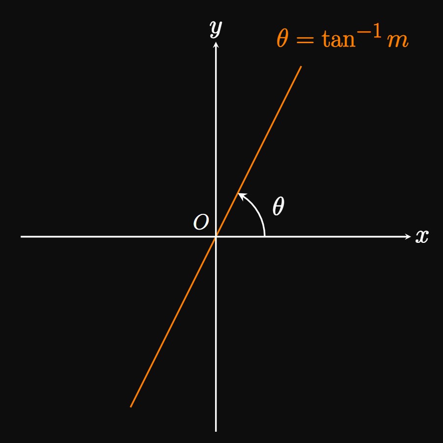
Suppose a line passes through the origin with slope \(m.\) Then the angle between the positive \(x\)-axis and the line is constant; hence, in polar form \(\theta\) is fixed, while \(r\) varies along the line. In Cartesian form, the equation of this line is \(y = mx.\) Dividing both sides by \(x\) gives \(m = y/x.\) Since \(\tan \theta = y/x,\) we have \(m = \tan \theta,\) or \begin{equation} \theta = \tan^{-1} m \pd \label{eq:polar-line} \end{equation} In words, this form asserts that the angle between the positive \(x\)-axis and a line that crosses the origin is the inverse tangent of the line's slope. (See Figure 11.)
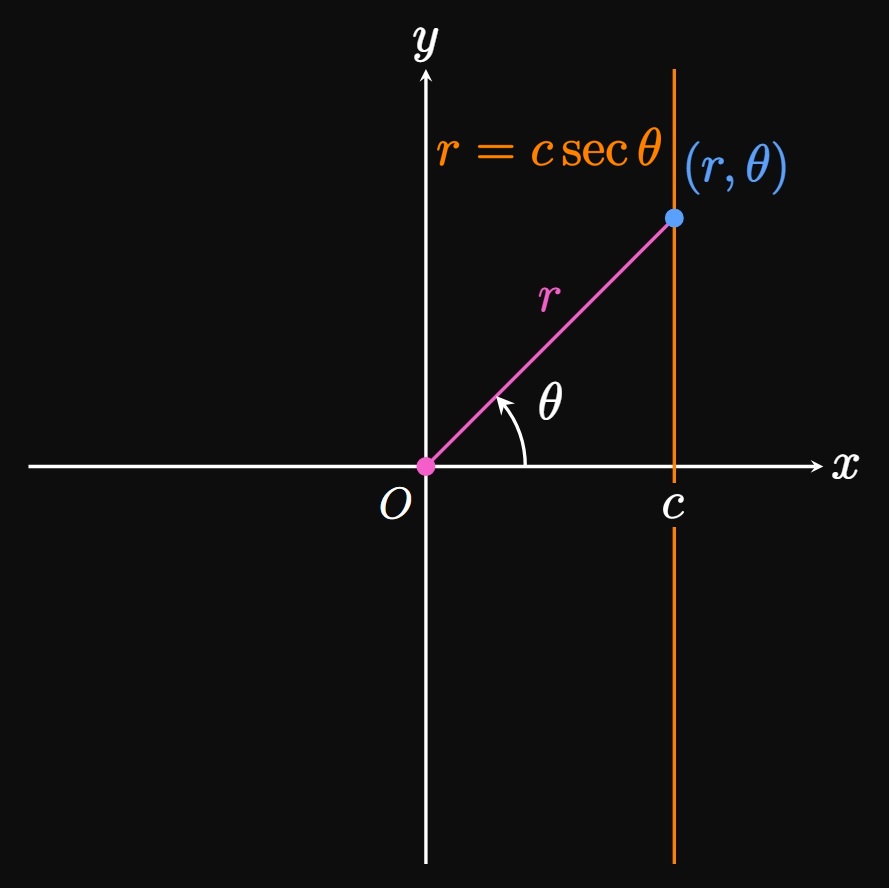
In Cartesian coordinates, a vertical line is of the form \(x = c.\) We convert this form to polar by replacing \(x\) with \(r \cos \theta\) and solving for \(r \col\) \begin{align} r \cos \theta &= c \nonumber \nl \implies r &= c \sec \theta \pd \label{eq:polar-vertical-line} \end{align} In Figure 12A, if you trace the vertical line upward—that is, as \(\theta\) approaches \(\pi/2\)—then \(r\) increases. In fact, \(\eqrefer{eq:polar-vertical-line}\) proves this observation because \(\lim_{\theta \to (\pi/2)^-} \abs{c \sec \theta} = \infty.\) Similarly, \(\lim_{\theta \to (-\pi/2)^+} \abs{c \sec \theta}\) \(= \infty,\) so the distance between the pole and the vertical line is increasing infinitely if you trace the vertical line downward. And when \(\theta = 0,\) the line segment connecting the pole to \((r, \theta)\) is a straight, horizontal line of length \(r = c.\)
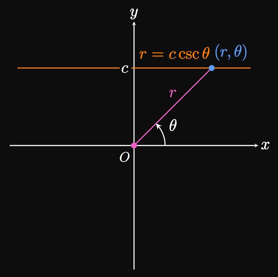
Through a similar procedure, we represent the horizontal line \(y = c\) in polar form by replacing \(y\) with \(r \sin \theta \col\) \begin{align} r \sin \theta &= c \nonumber \nl \implies r &= c \csc \theta \pd \label{eq:polar-horizontal-line} \end{align} (See Figure 12B.) As you trace the horizontal line in the direction of positive \(x,\) the angle \(\theta\) is shrinking to \(0.\) During this process the distance between the horizontal line and the point \(O\) is increasing to infinity, which we confirm by noting that \(\eqrefer{eq:polar-horizontal-line}\) satisfies \(\lim_{\theta \to 0^+} \abs{c \csc \theta} = \infty.\) Likewise, \(\lim_{\theta \to \pi^-} \abs{c \csc \theta} = \infty,\) so if we trace the horizontal line in the direction of negative \(x,\) then the distance between \(O\) and the horizontal line is also increasing to infinity. When \(\theta = \pi/2,\) the line segment connecting \(O\) to the point \((r, \theta)\) is vertical and has length \(r = c.\)
| Polar Equation | Cartesian Equation | Graph |
|---|---|---|
| \(\theta = \tan^{-1} m\) | \(y = mx\) | Line of slope \(m\) passing through origin |
| \(r = c \sec \theta\) | \(x = c\) | Vertical line |
| \(r = c \csc \theta\) | \(y = c\) | Horizontal line |
- \(\ds \theta = \frac{\pi}{3}\)
- \(r = 4 \csc \theta\)
- \(r = -2 \sec \theta\)
- Since \(\theta\) is fixed, this polar function represents a line. The line's slope \(m\) is \(\tan \theta,\) or \[m = \tan \frac{\pi}{3} = \sqrt 3 \pd\] In Cartesian form a line that passes through the origin with slope \(m\) is \(y = mx.\) Because \(m = \sqrt 3,\) we write the polar function in Cartesian form as \[\boxed{y = x \sqrt 3}\]
- The form \(r = c \csc \theta\) represents the horizontal line \(y = c.\) Here \(c = 4,\) so we write the expression in Cartesian form as \[\boxed{y = 4}\]
- The graph of \(r = c \sec \theta\) is the vertical line \(x = c.\) Thus, we write \(r = -2 \sec \theta\) in Cartesian form as \[\boxed{x = -2}\]
Spirals
Many graphs aren't expressed more easily in Cartesian coordinates. One example of a graph that is best expressed in polar form is a spiral (also called an Archimedean spiral).
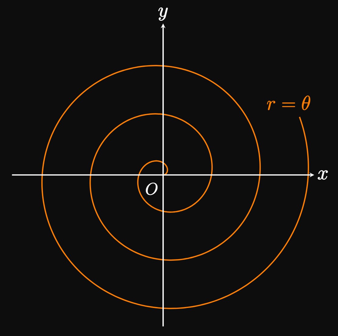
We now generalize this example. An Archimedean spiral is represented by the polar function \begin{equation} r = a + b \theta \pd \label{eq:polar-spiral} \end{equation} This form asserts that a particle's position from its starting point changes linearly with the angle \(\theta.\) Positive \(a\) shifts the spiral toward the positive \(x\)-axis, and negative \(a\) shifts the spiral toward the negative \(x\)-axis. The spiral in \(\eqref{eq:polar-spiral}\) curls in the counterclockwise direction if \(b \gt 0,\) and in the clockwise direction if \(b \lt 0.\) In Example 7, \(r\) increases as \(\theta\) increases—meaning each point on the graph of \(r = \theta\) grows farther away from the pole as we trace the angle \(\theta\) in the counterclockwise direction. So we say the graph of \(r = \theta\) curls in the counterclockwise direction.
If you wrap a strand of rope around your finger and spin your finger, then the uncoiling motion of the string forms a shape that resembles an Archimedean spiral. Attempting to write \(\eqrefer{eq:polar-spiral}\) as a Cartesian equation yields \[\sqrt{x^2 + y^2} = a + b \tan^{-1} \par{\frac{y}{x}} \cma \] a more complicated form. This form is very difficult to visualize, whereas \(\eqref{eq:polar-spiral}\) is much easier to understand.
- If \(a \gt 0,\) then the spiral begins at the positive \(x\)-axis. If \(a \lt 0,\) then the spiral begins at the negative \(x\)-axis.
- If \(b \gt 0,\) then the spiral curls in the counterclockwise direction. If \(b \lt 0,\) then the spiral curls in the clockwise direction.
Limacons and Cardioids
Polar graphs of the forms \[r = a + b \cos \theta \and r = a + b \sin \theta\] are called limacons. The graph of \(r = a + b \cos \theta\) is symmetric about the \(x\)-axis and is called a horizontal limacon. In contrast, a vertical limacon is symmetric about the \(y\)-axis and is represented by the function \(r = a + b \sin \theta.\) The following table provides additional information about each type of limacon.
| Polar Function | Graph |
|---|---|
| \(r = a + b \cos \theta\) | Horizontal limacon |
| \(r = a + b \sin \theta\) | Vertical limacon |
- If \(\abs a \geq \abs b,\) then the limacon has only one loop.
- If \(\abs a = \abs b,\) then the graph is called a cardioid, a heart-shaped limacon.
- If \(\abs a \lt \abs b,\) then the limacon has an inner loop.
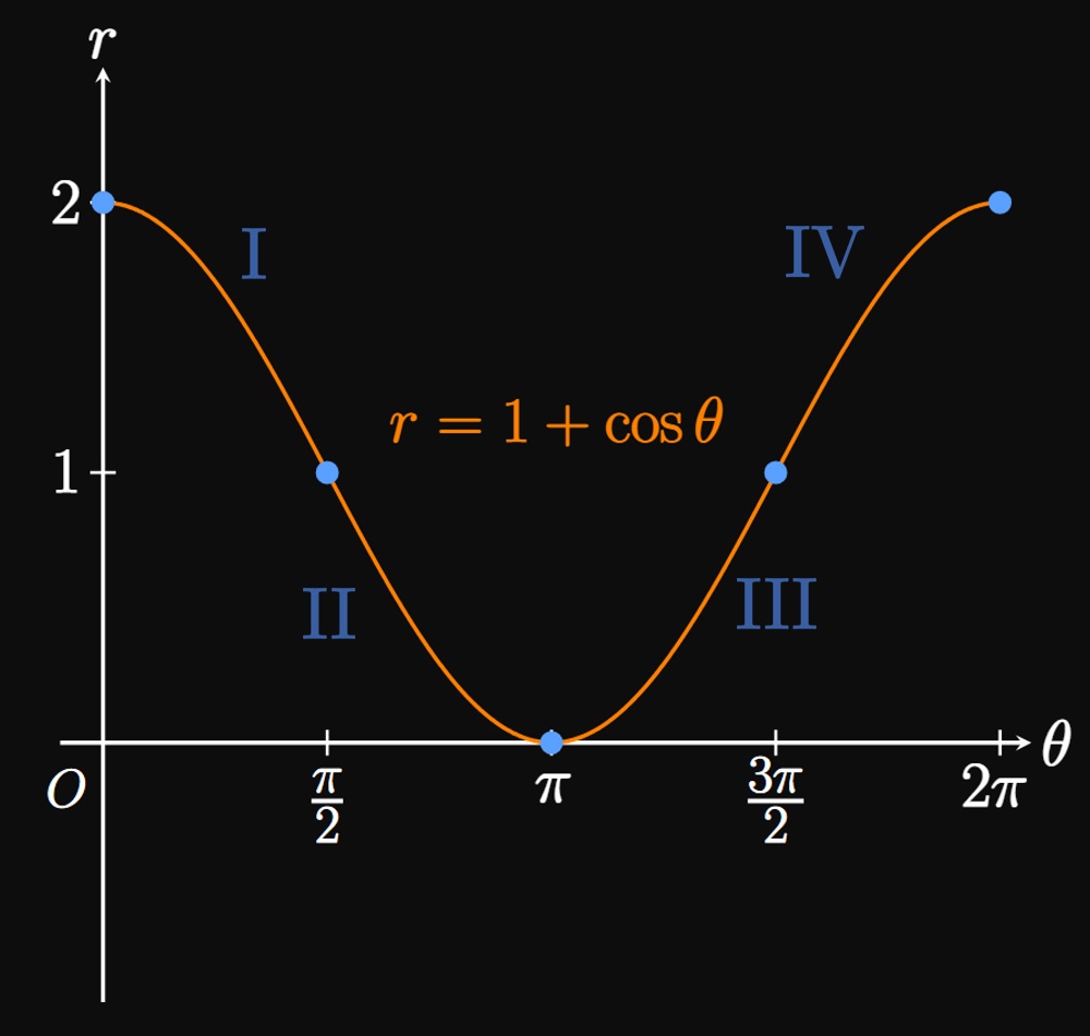
We need to determine how \(r\) varies with \(\theta\) to sketch the polar curve. It is easiest to first plot \(r = 1 + \cos \theta\) in Cartesian coordinates (Figure 14A). We note four key stages.
- As \(\theta\) increases from \(0\) to \(\pi/2,\) \(r\) decreases from \(2\) to \(1.\) Hence, two points on the polar curve are \((r, \theta) = (2, 0)\) and \((r, \theta) = (1, \pi/2).\) Note the decreasing distance between \((r, \theta)\) and the pole. We connect these points using an arc that extends through these points.
- Note that \(r = 0\) when \(\theta = \pi.\) Thus, the graph of the polar curve hits the origin when \(\theta = \pi.\) Since \(r\) is decreasing, the polar curve is getting closer to the origin. We therefore draw an arc that connects \((r, \theta)\) \(= \par{1, \pi/2}\) to \((r, \theta)\) \(= \par{0, \pi}.\)
- As \(\theta\) increases from \(\pi\) to \(3 \pi/2,\) \(r\) increases from \(0\) to \(1.\) Accordingly, on the polar curve we draw an arc connecting \((r, \theta)\) \(= \par{0, \pi}\) to \((r, \theta)\) \(= (1, 3\pi/2).\)
- The graph of \(r = 1 + \cos \theta\) finishes a complete revolution. So we close the loop on the polar graph.
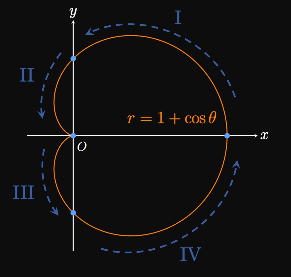
Alternatively, we could have noticed that, because cosine is an even function, \[1 + \cos \theta = 1 + \cos(-\theta) \pd\] Hence, the polar graph of \(r = 1 + \cos \theta\) is symmetric about the \(x\)-axis. So we could have traced the upper half of the graph \((0 \leq \theta \leq \pi)\) and mirrored it across the \(x\)-axis to obtain the bottom half of the graph \((\pi \leq \theta \leq 2\pi).\)
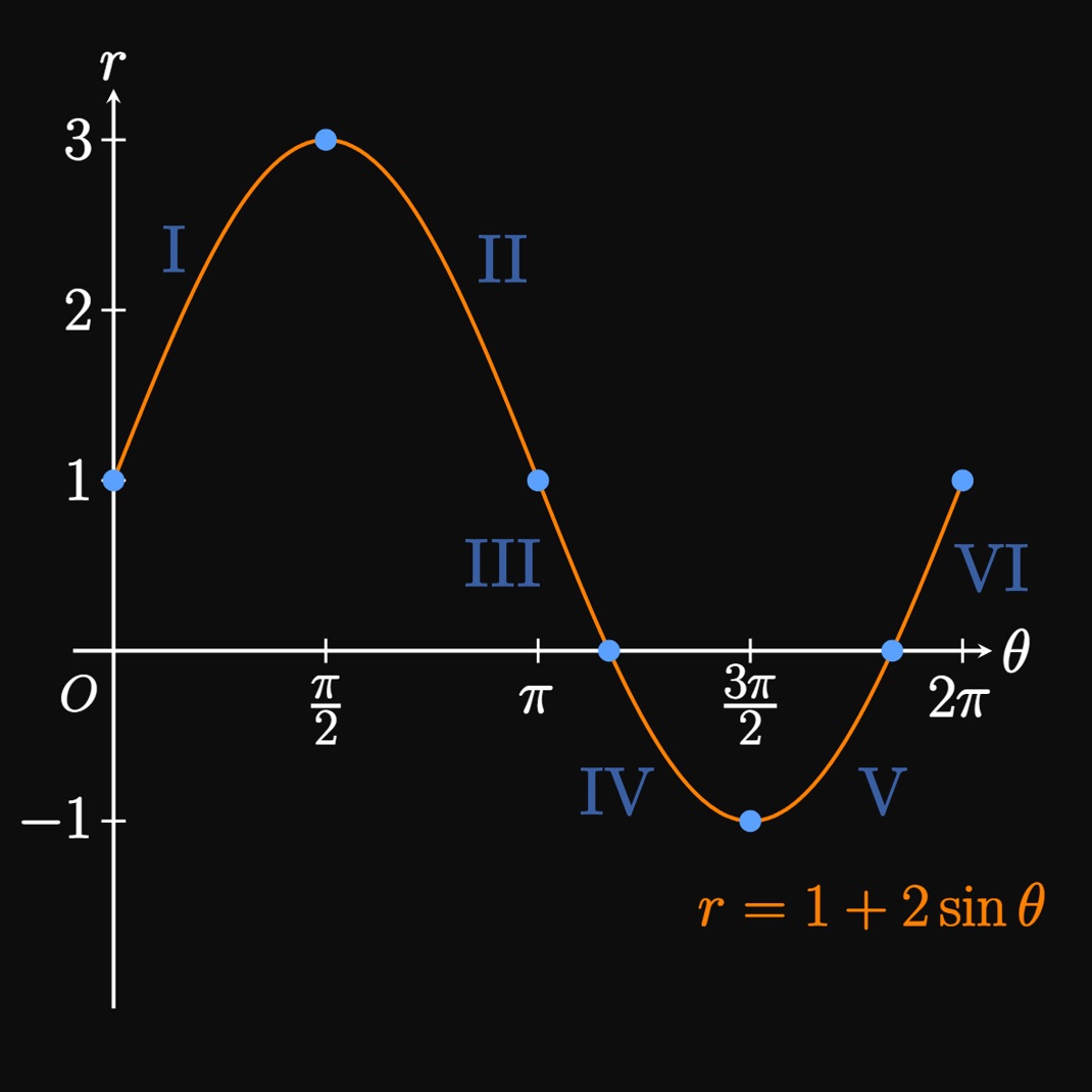
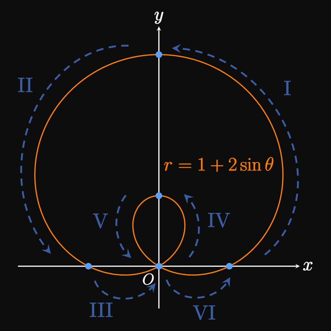
- As \(\theta\) increases from \(0\) to \(\pi/2,\) \(r\) increases from \(1\) to \(3.\) Thus, the polar graph of \(r = 1 + 2 \sin \theta\) passes through the points \((r, \theta) = (1, 0)\) and \((r, \theta) = (3, \pi/2).\) We therefore draw an arc that connects these points.
- As \(\theta\) increases from \(\pi/2\) to \(\pi,\) \(r\) decreases from \(3\) to \(1.\) So the polar curve passes through the points \((r, \theta) = (3, \pi/2)\) and \((r, \theta) = (1, \pi).\)
- The Cartesian graph of \(r = 1 + 2 \sin \theta\) has a zero when \(\theta = 7 \pi/6.\) The polar graph therefore crosses the pole when \(\theta = 7 \pi/6.\) So we connect the point \((r, \theta) = (1, \pi)\) to \((r, \theta) = (0, 7 \pi/6).\)
- As \(\theta\) increases from \(7 \pi/6\) to \(3 \pi/2,\) \(r\) decreases from \(0\) to \(-1.\) Accordingly, the polar curve passes through \((r, \theta) = (-1, 3\pi/2).\) Since \(r \lt 0,\) this point is a reflection of the point \((1, 3 \pi/2)\) by \(\pi\) radians—giving us a point on the positive \(y\)-axis.
- Note that \(r = 0\) when \(\theta = 11 \pi/6.\) So we draw an arc connecting the polar curve from \((r, \theta) = (-1, 3\pi/2)\) to the pole at \(\theta = 11 \pi/6.\) Steps IV and V trace an inner loop of the graph.
- Because \((r, \theta) = (1, 2 \pi)\) represents the same point as \((r, \theta) = (1, 0),\) we close the graph of the polar curve.
Roses
The polar graph of \begin{equation} r = \cos n \theta \or r = \sin n \theta \label{eq:polar-rose} \end{equation} forms a rose whose center is at the origin. We consider \(n\) to be a positive integer. Then we have two cases: when \(n\) is odd and when \(n\) is even. If \(n\) is odd, then the graph of either function in \(\eqref{eq:polar-rose}\) has \(n\) petals (Figure 16A). Conversely, if \(n\) is even, then either graph in \(\eqref{eq:polar-rose}\) has \(2 n\) petals (Figure 16B).
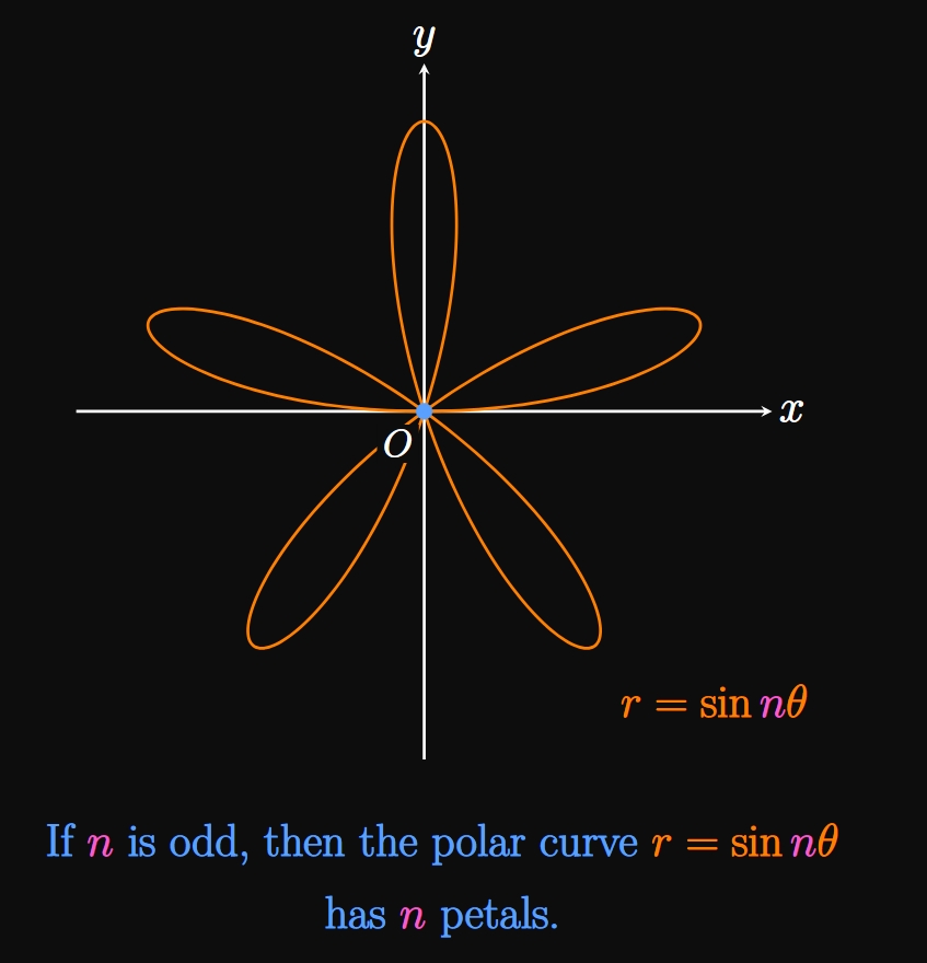
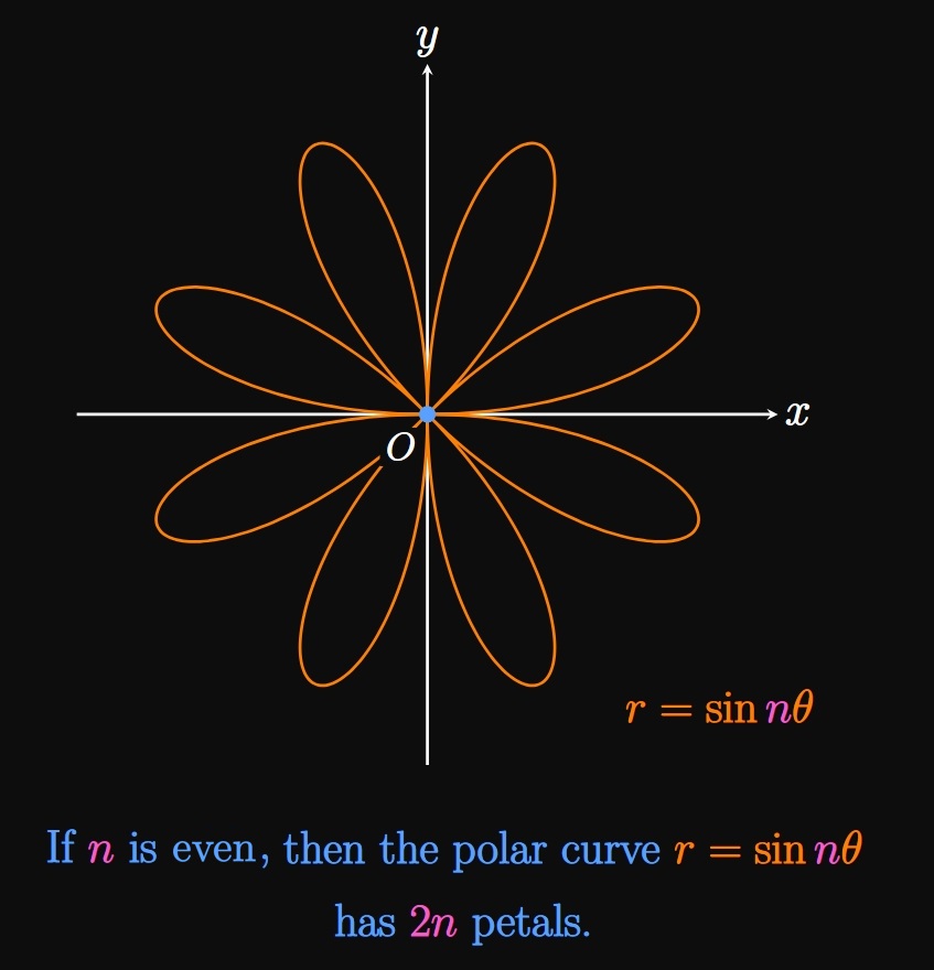
- If \(n\) is odd, then the graph has \(n\) petals.
- If \(n\) is even, then the graph has \(2n\) petals.
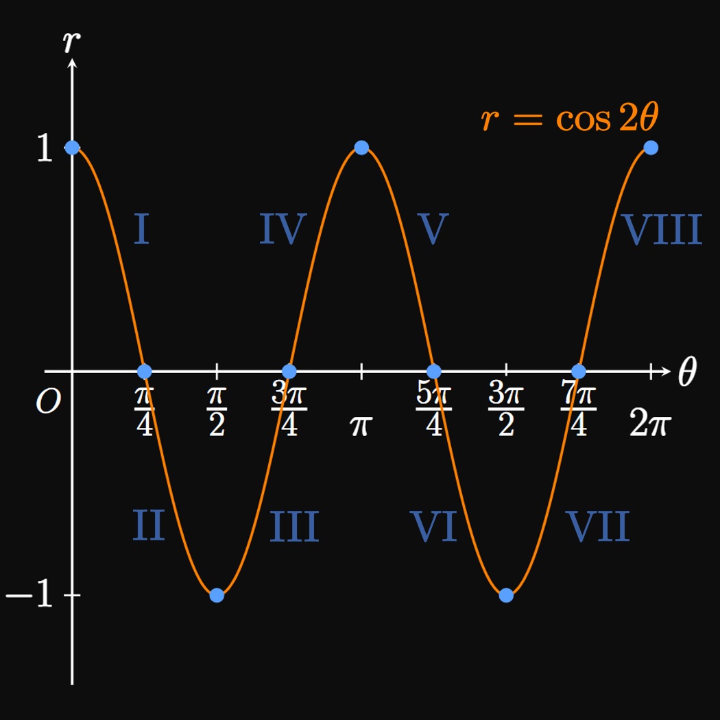
We first plot the graph of \(r = \cos 2 \theta\) in Cartesian coordinates (Figure 17A). We analyze eight stages.
- As \(\theta\) increases from \(0\) to \(\pi/4,\) \(r\) decreases from \(1\) to \(0.\) Hence, on the polar curve \(r = \cos 2 \theta\) we plot two points: \((r, \theta) = (1, 0)\) and \((r, \theta) = (0, \pi/4).\) The arc connecting these points forms half a petal.
- For \(\theta \in (\pi/4, \pi/2),\) \(r\) is negative and drops to \(-1\) when \(\theta = \pi/2.\) The points on the polar graph therefore lie on the opposite side of the first quadrant—in the third quadrant, forming a half-petal that begins at the origin and terminates at the ray \(\theta = 3 \pi/2.\)
- As \(\theta\) increases from \(\pi/2\) to \(3 \pi/4,\) \(r\) increases from \(-1\) to \(0.\) Since \(r\) is negative in this interval, the points on the polar curve reside in the fourth quadrant instead of in the second quadrant. These points trace a half-petal that starts at the ray \(\theta = 3\pi/2\) and ends at the origin. Stages II and III form a full petal of the graph on the negative \(y\)-axis.
- As \(\theta\) increases from \(3 \pi/4\) to \(\pi,\) \(r\) increases from \(0\) to \(1.\) Thus, points on the polar graph of \(r = \cos 2 \theta\) trace a half-petal in the second quadrant that begins at the origin and terminates at the ray \(\theta = \pi.\)
- As \(\theta\) increases from \(\pi\) to \(5 \pi/4,\) \(r\) decreases from \(1\) to \(0.\) Accordingly, in the third quadrant the polar graph of \(r = \cos 2 \theta\) traces a half-petal that begins at the ray \(\theta = \pi\) and ends at the origin. Stages IV and V therefore form a full petal that resides on the negative \(x\)-axis.
- The polar graph passes through \((r, \theta) = (0, 5 \pi/4)\) and \((r, \theta) = (-1, 3\pi/2).\) Since \(r \lt 0,\) instead of the points tracing an arc in the third quadrant, they form an arc in the first quadrant that begins at the origin and ends at the positive \(y\)-axis.
- Now \(r\) increases from \(-1\) to \(0\) as \(\theta\) increases from \(3\pi/2\) to \(7 \pi/4.\) Because \(r \lt 0,\) the arc of the polar graph—instead of residing in the fourth quadrant—traces out a half-petal in the second quadrant. Stages VI and VII trace a full petal that lies on the positive \(y\)-axis.
- The polar graph passes through the points \((r, \theta) = (0, 7\pi/4)\) and \((r, \theta) = (1, 2\pi).\) Hence, this last arc culminates the petal that lies on the positive \(x\)-axis.
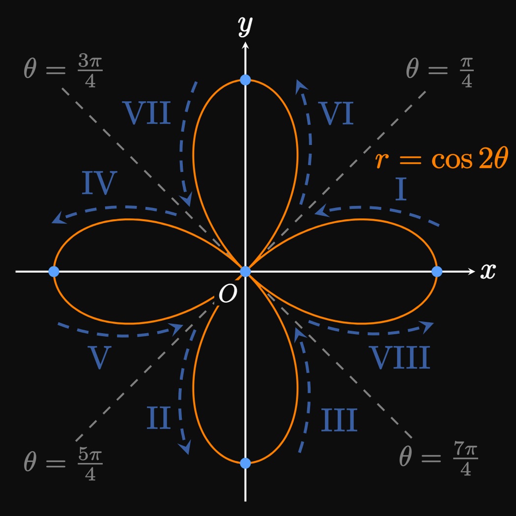
Alternatively, a simpler option is to exploit the symmetry of the graph: The curve is symmetric about the \(x\)-axis because \[\cos 2 \theta \equalsCheck \cos(-2 \theta) \pd\] It is also symmetric about the \(y\)-axis since \[\cos 2 \theta \equalsCheck \cos[2(\pi - \theta)] \pd\] From these remarks, we can sketch the half-petal in stage I, reflect a copy across the \(x\)-axis (obtaining VIII), and then reflect both halves across the \(y\)-axis (to get IV and V). Doing so gives us the two petals that lie on the \(x\)-axis. To obtain the vertical petals, we can sketch stage II of the polar graph. Reflecting a copy of this half-petal across the \(y\)-axis gives III, and reflecting both halves across the \(x\)-axis yields portions VII and VI. This entire procedure covers all values of \(\theta\) and therefore produces the full graph of \(r = \cos 2 \theta.\) When we apply symmetry, we must ensure that our strategy covers all values of \(\theta;\) otherwise, we may miss portions of the graph.
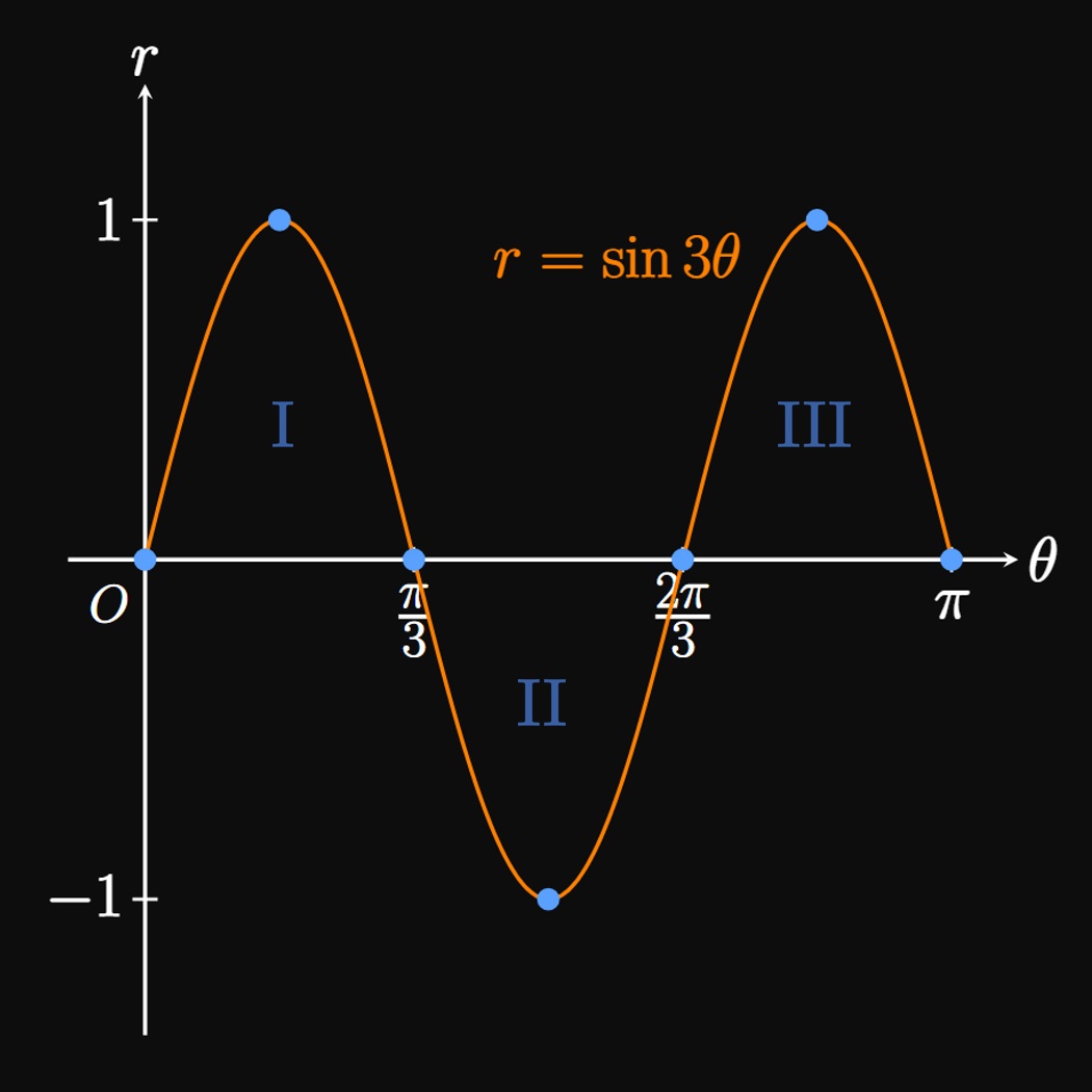
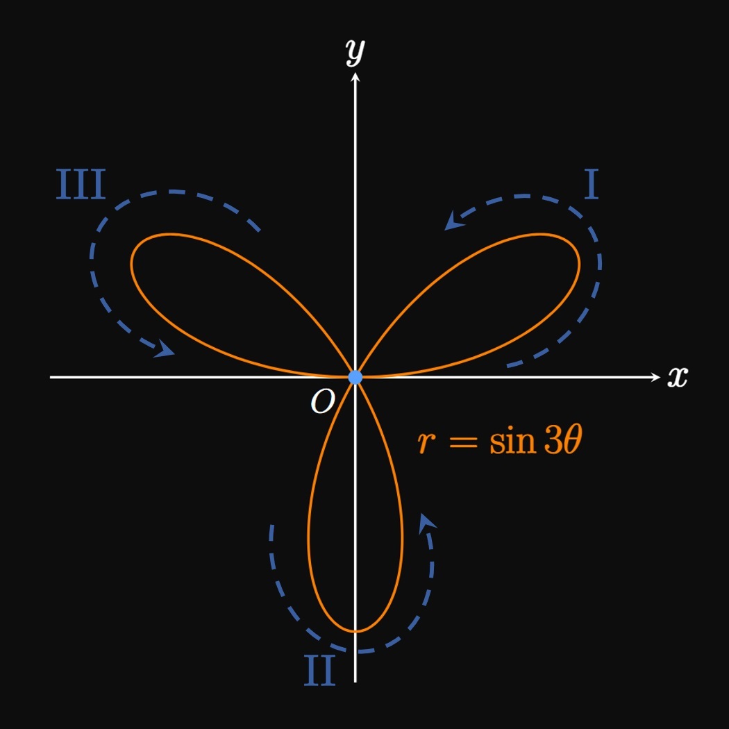
- The polar graph passes through the origin when \(\theta = 0\) since \(r = 0.\) Then \(r\) increases to \(1\) when \(\theta = \pi/6,\) before falling to \(0\) when \(\theta = \pi/3.\) Accordingly, for the polar curve \(r = \sin 3 \theta\) we trace a petal in the first quadrant that intersects the origin at \(\theta = 0\) and \(\theta = \pi/3,\) with a vertex occurring when \(\theta = \pi/6.\)
- For \(\pi/3 \lt \theta \lt 2 \pi/3,\) \(r\) is negative. The polar graph therefore enters the third and fourth quadrants. For \(\pi/3 \leq \theta \leq \pi/2\) we trace a half-petal in the third quadrant, and for \(\pi/2 \leq \theta \leq 2 \pi/3\) we draw the other half of the petal in the fourth quadrant. Doing so yields a petal along the negative \(y\)-axis.
- For \(2 \pi/3 \lt \theta \lt \pi,\) \(r\) is positive. Hence, in the second quadrant we draw a petal that strikes the origin when \(\theta = 2 \pi/3\) and \(\theta = \pi.\)
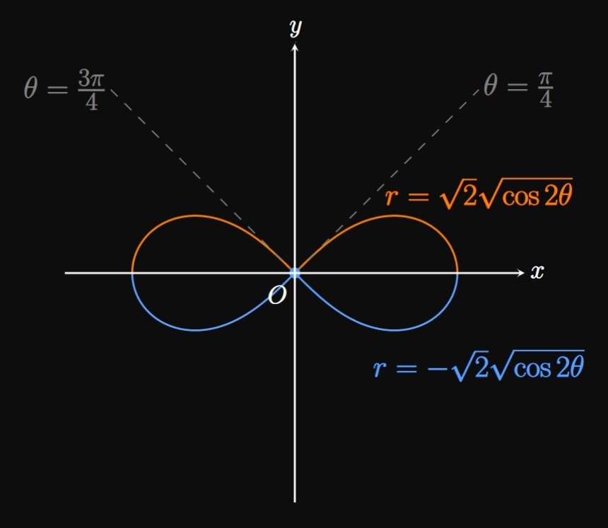
Lemniscates
A lemniscate is an \(\infty\)-shaped curve. It is formed by either equation \[r^2 = a^2 \cos 2 \theta \or r^2 = a^2 \sin 2 \theta \pd \] We graph a lemniscate by splitting \(r^2\) into two functions of \(r\)—one positive and one negative. Graphing both functions yields the full lemniscate.
Polar Coordinates Polar coordinates represent a point in a plane as \((r, \theta).\) Here, \(r\) is the length of the line that connects the pole (the origin) to point \((r, \theta),\) and \(\theta\) is the angle between the polar axis—the positive \(x\)-axis—and \((r, \theta).\) The angle \(\theta\) is positive if it extends in the counterclockwise direction and negative if it extends in the clockwise direction. If \(r\) is replaced by \(-r,\) then the line segment that connects \(O\) to \((r, \theta)\) is rotated \(\pi\) radians about the origin; this new point is denoted as \((-r, \theta)\) or \((r, \theta + \pi).\) We convert between polar and Cartesian forms by using \(x = r \cos \theta,\) \(y = r \sin \theta,\) \(r^2 = x^2 + y^2,\) and \(\tan \theta = y/x.\) A polar function expresses \(r\) as a function of \(\theta\)—namely, \(r = f(\theta).\)
Symmetry with Polar Functions Let \(f\) be a polar function. Then the following properties of symmetry apply.
- If \(f(\theta) = f(-\theta),\) then the graph of \(r = f(\theta)\) is symmetric about the \(x\)-axis.
- If \(f(\theta) = f(\pi -\theta),\) then the graph of \(r = f(\theta)\) is symmetric about the \(y\)-axis.
- If \(f(\theta) = -f(\theta + \pi),\) then the graph of \(r = f(\theta)\) is symmetric about the origin.
| Polar Equation | Cartesian Equation | Graph |
|---|---|---|
| \(r = k\) | \(x^2 + y^2 = k^2\) | Circle of radius \(|k|\) centered at origin |
| \(r = k \cos \theta\) | \(\ds \par{x - \frac{k}{2}}^2 + y^2 = \frac{k^2}{4}\) | Circle of radius \(|k/2|\) centered at \((x, y) = (k/2, \, 0)\) |
| \(r = k \sin \theta\) | \(\ds x^2 + \par{y - \frac{k}{2}}^2 = \frac{k^2}{4}\) | Circle of radius \(|k/2|\) centered at \((x, y) = (0, \, k/2)\) |
| Polar Equation | Cartesian Equation | Graph |
|---|---|---|
| \(\theta = \tan^{-1} m\) | \(y = mx\) | Line of slope \(m\) passing through origin |
| \(r = c \sec \theta\) | \(x = c\) | Vertical line |
| \(r = c \csc \theta\) | \(y = c\) | Horizontal line |
Spirals A spiral (or Archimedean spiral) is the graph of \(r = a + b \theta,\) where \(a\) and \(b\) are constants.
- If \(a \gt 0,\) then the spiral begins at the positive \(x\)-axis. If \(a \lt 0,\) then the spiral begins at the negative \(x\)-axis.
- If \(b \gt 0,\) then the spiral curls in the counterclockwise direction. If \(b \lt 0,\) then the spiral curls in the clockwise direction.
Limacons and Cardioids The graphs of \(r = a + b \cos \theta\) and \(r = a + b \sin \theta\) are limacons.
| Polar Function | Graph |
|---|---|
| \(r = a + b \cos \theta\) | Horizontal limacon |
| \(r = a + b \sin \theta\) | Vertical limacon |
- If \(\abs a \geq \abs b,\) then the limacon has only one loop.
- If \(\abs a = \abs b,\) then the graph is called a cardioid, a heart-shaped limacon.
- If \(\abs a \lt \abs b,\) then the limacon has an inner loop.
Roses The graphs of \(r = \cos n \theta\) and \(r = \sin n \theta,\) where \(n\) is a positive integer, form roses. If \(n\) is odd, then the graph has \(n\) petals; if \(n\) is even, then the graph has \(2n\) petals.
Lemniscates The graphs of \(r^2 = a^2 \cos 2 \theta\) and \(r^2 = a^2 \sin 2\theta\) are lemniscates. A lemniscate is an \(\infty\)-shaped curve. We graph a lemniscate by splitting \(r^2\) into two functions of \(r\)—one positive and one negative—and graphing each.