3.7: Applications of Differentiation in Economics
Many customers are willing to purchase a new phone for \(\$100,\) but fewer are willing to pay \(\$900\) for the same phone. A manufacturer must therefore lower the phone's price to increase sales. In general, as an item's price is raised, fewer consumers demand that product. This inverse relationship between price and the number of units demanded is called the Law of Demand. But how much should a product cost if a store wants to sell \(x\) units? In economics, we use a demand function \(p(x)\) to model the price per unit that a firm can charge to sell \(x\) units. Because revenue is the product of price and the number of units sold, a firm's revenue function is defined by \begin{equation} R(x) = x \, p(x) \pd \label{eq:revenue-R} \end{equation} For example, a movie theater's revenue could increase if ticket prices are raised or if more tickets are sold.
Cost Functions To produce additional goods, a business must pay to expand. For example, a small electronics chain may easily sell \(50\) phones per day; but to sell \(500\) phones per day, the store must expand its inventory, hire additional employees, and pay for advertisements—thus incurring additional costs passed on to the phones' prices. So a firm's cost function \(C(x),\) its cost to produce \(x\) units, is usually increasing. Then a firm's profit function is given by the difference between revenue and cost: \begin{equation} P(x) = R(x) - C(x) \pd \label{eq:profit-P} \end{equation} A negative profit indicates that a firm is losing money.
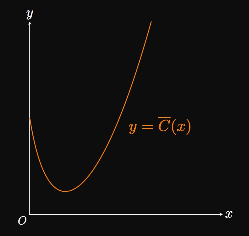
A firm's average cost function, the average cost per unit produced, is defined by \begin{equation} \overline C(x) = \frac{C(x)}{x} \cmaa x \gt 0 \pd \label{eq:avg-cost} \end{equation} We expect the graph of \(y = \overline C(x)\) to be concave up and have an absolute minimum (Figure 1). Initially, a firm incurs high startup costs (such as purchasing a store location), resulting in a high average cost per unit produced. But this initial investment enables the firm to sell more units, so the average cost per unit begins decreasing. Eventually, the firm reaches a point at which its resources are strained and must invest further to increase its capacity for production, such as by opening a new location. Consequently, as production continues to grow, the average cost increases.
Marginal analysis explores a firm's additional gains or losses from producing one more unit. Let's take the cost function \(C(x)\) to be differentiable. Even though \(x\) usually takes on integer values (to represent the number of goods sold), the differentiability assumption enables us to use calculus to attain useful results. Suppose that the number of products sold increases from \(x_1\) to \(x_2,\) and let \(\Delta x = x_2 - x_1.\) Then the average rate of change of \(C\) on \([x_1, x_2]\) is \[\frac{\Delta C}{\Delta x} = \frac{C(x_2) - C(x_1)}{x_2 - x_1} = \frac{C(x_1 + \Delta x) - C(x_1)}{\Delta x} \pd\] Then the cost function's instantaneous rate of change at \(x_1\) is \[C'(x_1) = \lim_{\Delta x \to 0} \frac{C(x_1 + \Delta x) - C(x_1)}{\Delta x} \pd\] We call \(C'(x)\) the marginal cost function; it approximates the cost to produce one more unit. If a firm produces \(n\) units, then we estimate \[C'(n) \approx \underbrace{C(n + 1) - C(n)}_{\text{cost of } (n + 1)\text{st unit}} \pd\] This approximation is especially accurate for large \(n.\) Using similar logic, we define the marginal revenue function to be \(R'(x)\) and the marginal profit function to be \(P'(x).\) If marginal profit is positive, then the firm should produce an extra unit. Yet if marginal profit is negative, then the firm should stop expanding production to avoid further losses.
In the next examples, we maximize firms' profits. See Section 3.1 to review the procedure of determining absolute maxima. In a competitive market with many buyers, a business's demand function can often be approximated as constant, as shown by the following example.
The Law of Demand explains an inverse relationship between a good's price and the quantity demanded of the good. The demand function \(p(x)\) models the price per unit at which \(x\) units are sold. The firm's revenue function is the product of quantity and price: \begin{equation} R(x) = x \, p(x) \pd \eqlabel{eq:revenue-R} \end{equation} A firm's cost function \(C(x)\) models the cost incurred to produce \(x\) units; it is an increasing function. The profit function is the difference between revenue and cost: \begin{equation} P(x) = R(x) - C(x) \cma \eqlabel{eq:profit-P} \end{equation} where a negative profit indicates a net loss. The average cost function is \begin{equation} \overline C(x) = \frac{C(x)}{x} \cmaa x \gt 0 \pd \eqlabel{eq:avg-cost} \end{equation} We expect the average cost function to be concave up and have an absolute minimum. A firm's marginal cost function \(C'(x)\) predicts the cost of producing the next unit. Likewise, the marginal revenue function \(R'(x)\) predicts the revenue attained by producing an additional unit, and the marginal profit function is \(P'(x) = R'(x) - C'(x).\) If the marginal profit is negative, then the firm should not produce an additional unit.