5.1: Areas between Curves
In Section 4.2 we calculated areas of regions bounded between a function and the \(x\)-axis. But we now compute areas of regions bounded between two or more functions. In doing so, we discuss the following:
Areas with \(x\)
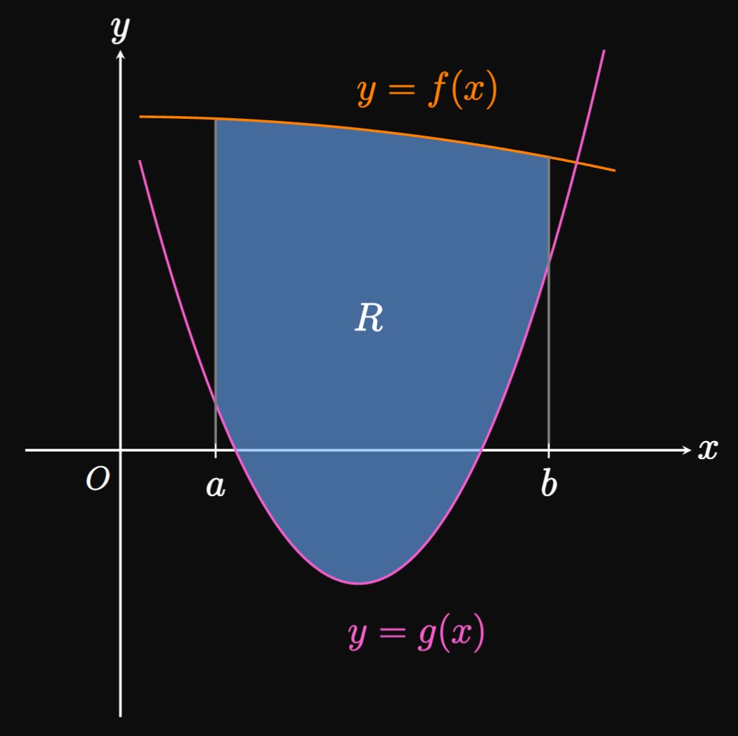
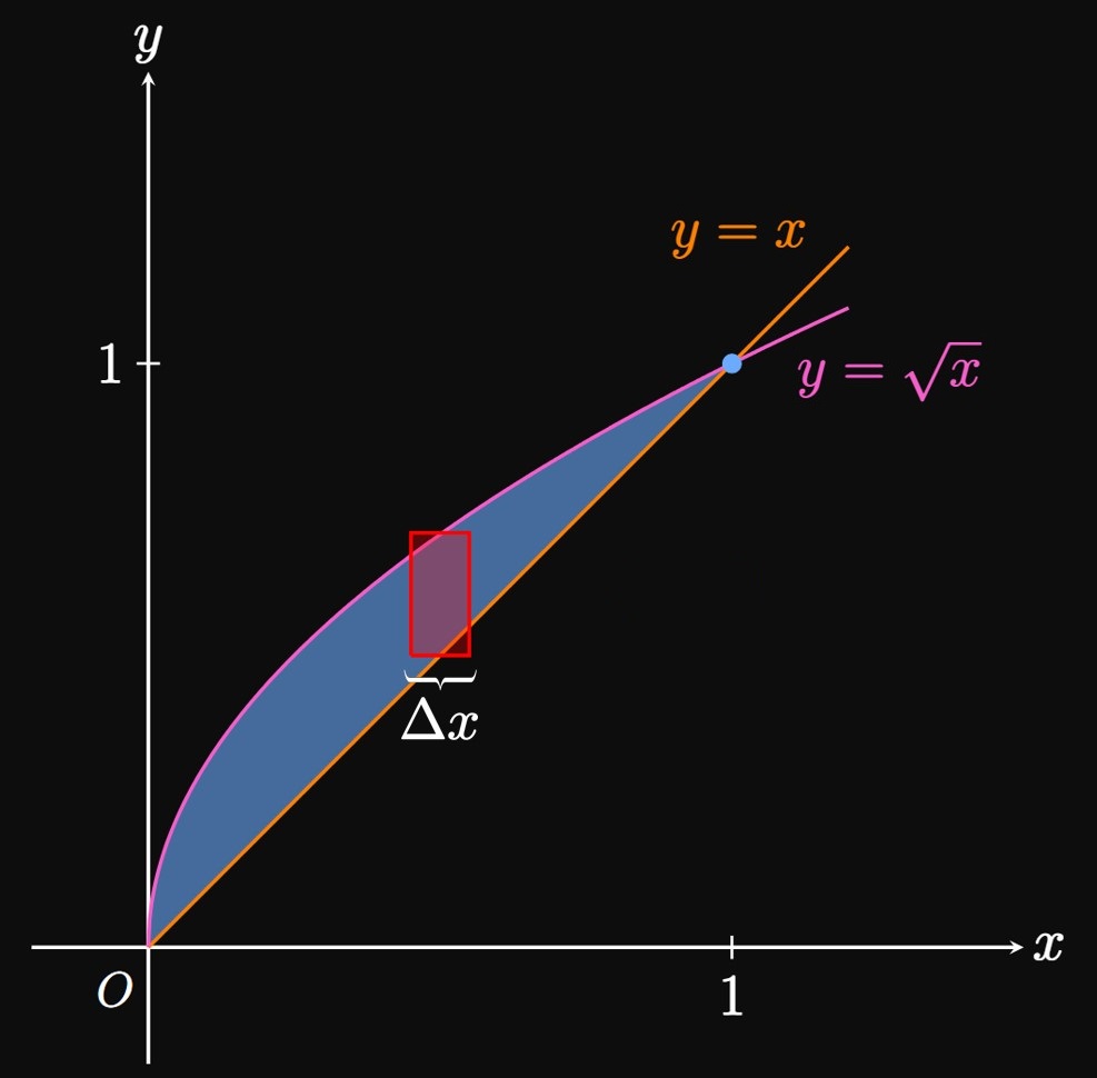
In Figure 1, region \(R\)
is bounded between two continuous functions \(f(x)\) and \(g(x)\)
and between the lines \(x = a\) and \(x = b.\)
We proceed by assuming that \(f(x) \geq g(x)\) for all \(x\) in \([a, b].\)
To find the area, we construct a Riemann sum in which we cut \(R\) into \(n\)
rectangles of equal width \(\Delta x.\)
The height of the
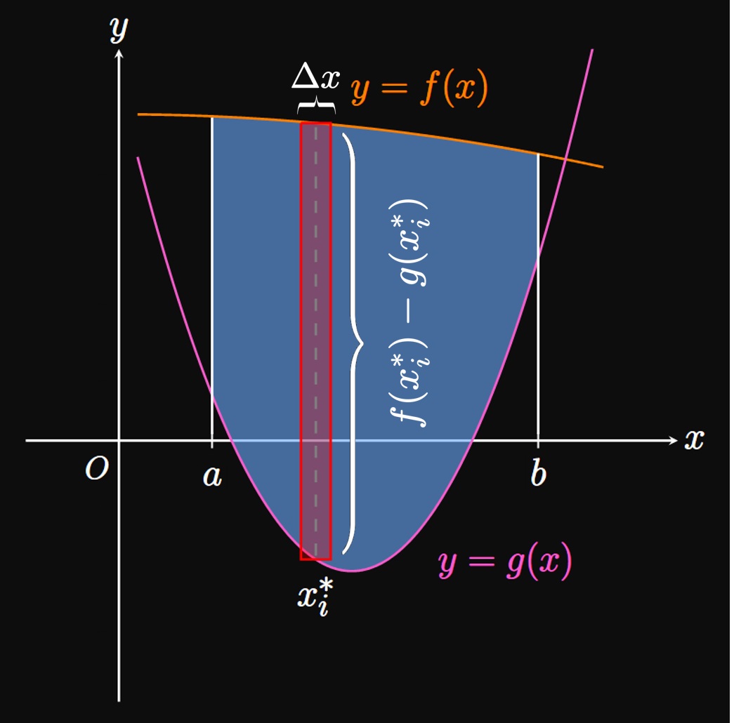
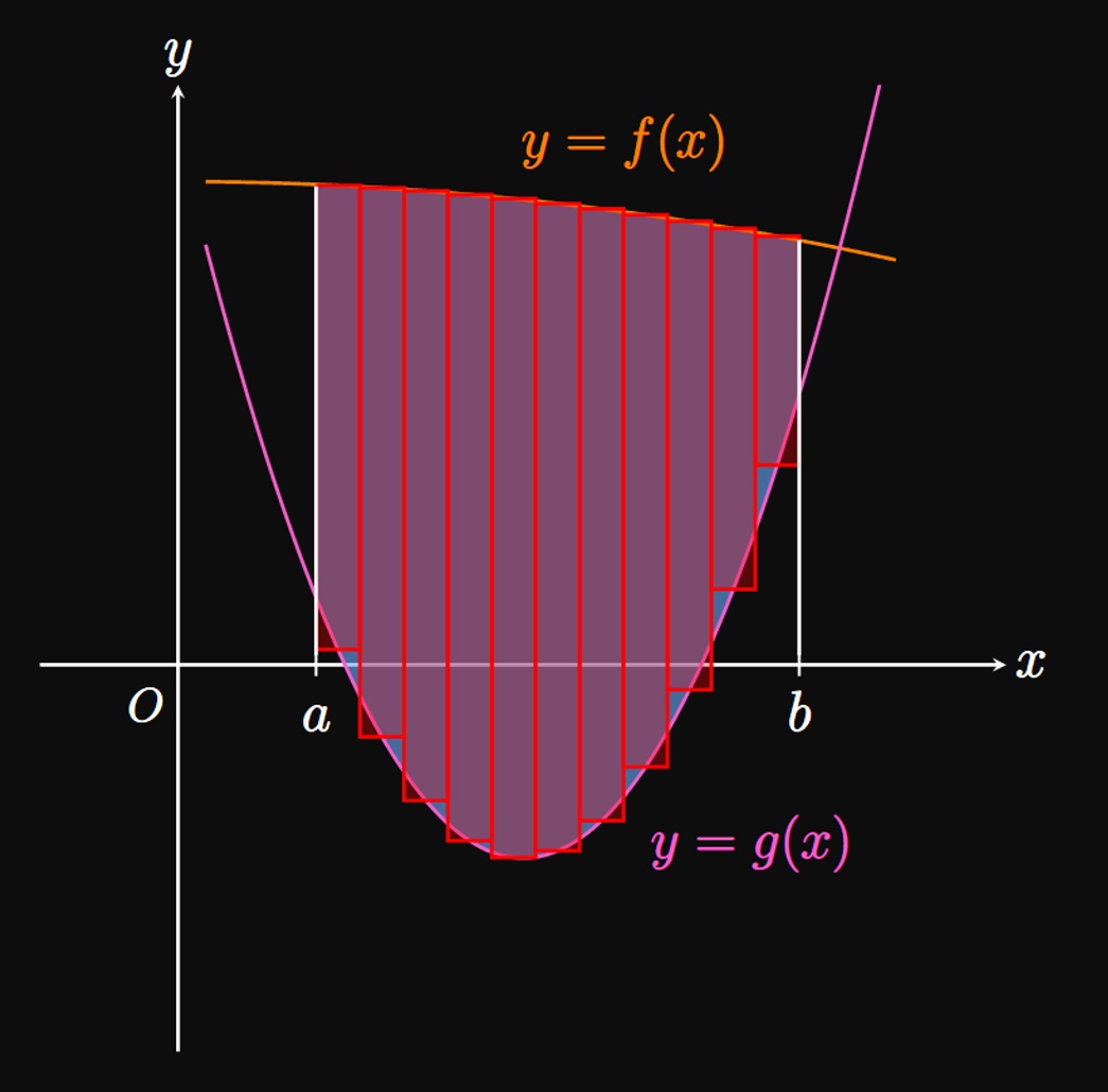
As in Figure 2B, we wish to sum up \(n\) of these rectangles to approximate the area \(A.\) As \(n\) is increased, the rectangles become thinner and therefore better approximate \(A.\) Our Riemann sum is therefore \[A = \lim_{n \to \infty} \sum_{i = 1}^n [f(x_i^*) - g(x_i^*)] \, \Delta x \pd\] This limit is the definite integral of \(f(x) - g(x),\) so we have \begin{equation} A = \int_a^b [f(x) - g(x)] \di x \pd \label{eq:area-x} \end{equation}
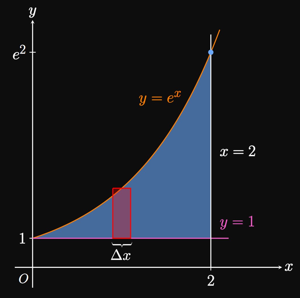
In the special case where \(f\) and \(g\) are both positive,
\(\eqref{eq:area-x}\) asserts that the area between the graphs is the
area under \(f\) minus the area under \(g.\)
That is,
\[
\ba
A &= [\textrm{area under} \; y = f(x)] - [\textrm{area under} \; y = g(x)] \nl
&= \int_a^b f(x) \di x - \int_a^b g(x) \di x \nl
&= \int_a^b [f(x) - g(x)] \di x \pd
\ea
\]
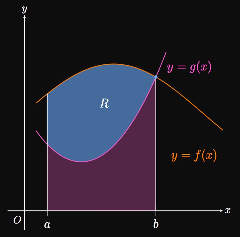
See Figure 3:
the pink area under the graph of \(g\) is subtracted from the total orange area under the graph of \(f.\)
Informally, \(\eqref{eq:area-x}\) says we integrate the top function
minus the bottom function, or top minus bottom,
to calculate areas of bounded regions.
When we solve problems, we need to visualize the situation. Thus, always draw a sketch of the bounded area in question. Before you integrate, ensure that in the bounded area one function is greater than the other. Note that \(\eqref{eq:area-x}\) should never return a negative result; the area of an enclosed region is independent of the quadrant in which it lies.
To use \(\eqref{eq:area-x},\) we need \(f(x) \geq g(x)\) for all \(x\) in \([a, b].\) But if \(g(x) \geq f(x)\) for some \(x\) in this interval, then we use the absolute value of the difference: \[A = \int_a^b \abs{f(x) - g(x)} \di x \pd\] Mathematically, this procedure is equivalent to splitting the region \(R\) into subregions; in each, one function is greater than the other. The following example shows this principle.
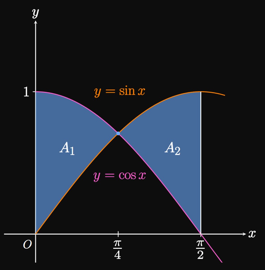
REMARK Mathematically, this procedure works because \[ \ba \int_{0}^{\pi/2} \abs{\cos x - \sin x} \di x &= \int_0^{\pi/4} \par{\cos x - \sin x} \di x + \int_{\pi/4}^{\pi/2} \par{\sin x - \cos x} \di x \nl &= A_1 + A_2 \pd \ea \]
Areas with \(y\)
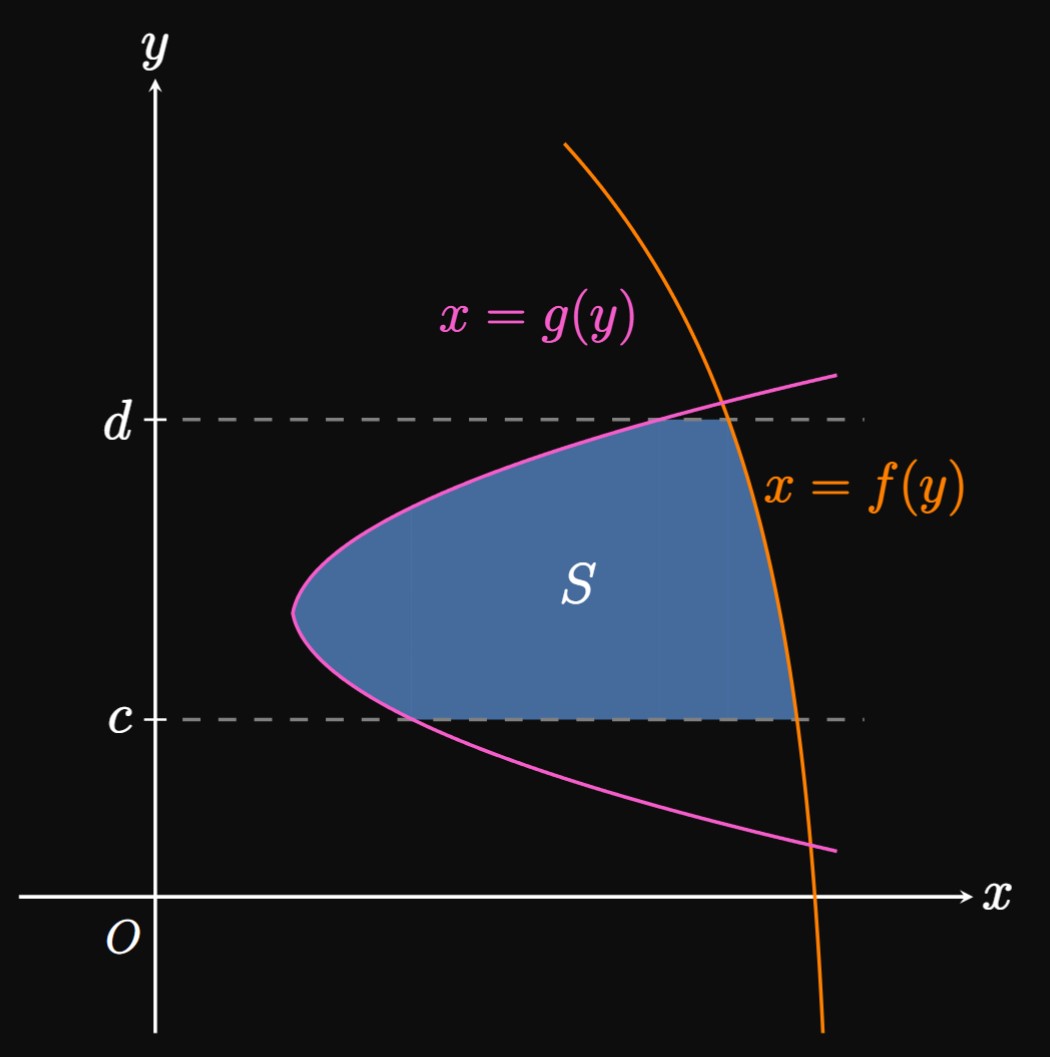
We may wish to find areas bounded by functions of \(y.\) In Figure 7, region \(S\) is bounded by the functions \(x = f(y)\) and \(x = g(y)\) as well as by the horizontal lines \(y = c\) and \(y = d.\) To compute this area, we arrange Riemann sums in which the rectangles are horizontal; Figure 8A shows a typical rectangle in this scenario. The rectangle's area is the height \(\Delta y\) multiplied by the length \(f(y_i^*) - g(y_i^*).\) Note that since the graph of \(f\) is to the right of \(g,\) \(x = f(y)\) takes on greater values of \(x\) than does \(x = g(y).\) Accordingly, the difference \(f - g\) is a positive quantity.
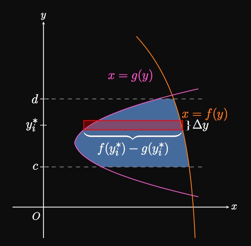
The Riemann sum for infinitely many rectangles,
if \(f(y) \geq g(y)\) for \(c \leq y \leq d,\) is
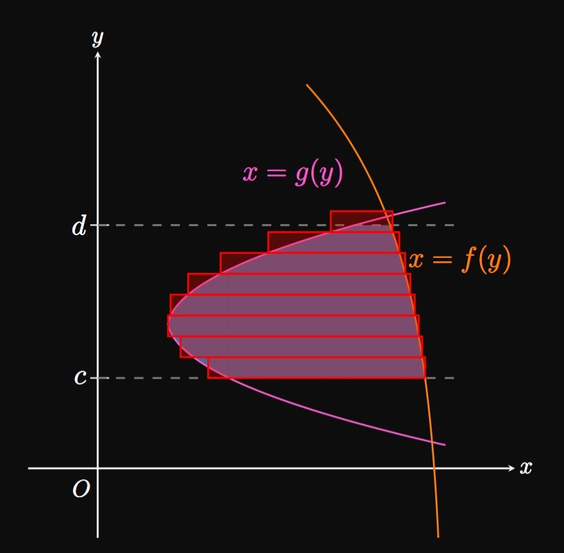
\[A = \lim_{n \to \infty} \sum_{i = 1}^n [f(y_i^*) - g(y_i^*)] \, \Delta y \pd\]
(See Figure 8B.)
This limit is the definite integral
\begin{equation}
A = \int_c^d [f(y) - g(y)] \di y \pd \label{eq:area-y}
\end{equation}
When we integrate a region with respect to \(y,\) we use right minus left
instead of top minus bottom,
as we do with Areas with \(x\).
Integrating horizontally may be unfamiliar to you.
If so, you may find it helpful to rotate the graph counterclockwise such that
the horizontal cuts become rotated, vertical strips.
Doing so shows a parallel between heights in Areas with \(x\)
and widths in areas integrated with \(y.\)
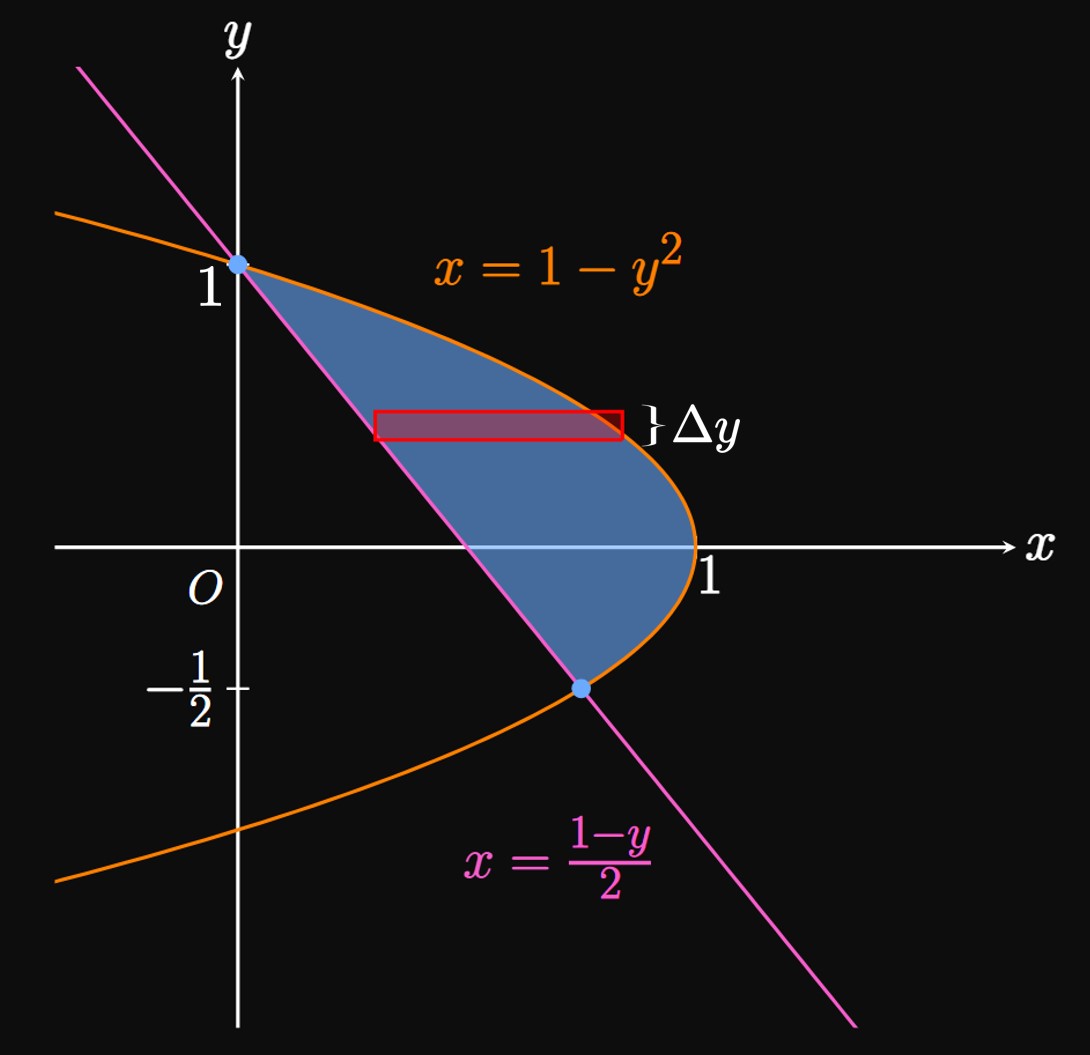
After sketching the bounded area (Figure 9), it's apparent that slicing the region vertically (that is, integrating with respect to \(x\)) would be very difficult. But cutting the region horizontally (integrating with respect to \(y\)) is convenient because the function \(1 - y^2\) is to the right of the line \((1 - y)/2\) for all \(y\) in our region. This means the boundaries are the same functions, so we can just write one integral. We are given the intersection points, so we apply \(\eqref{eq:area-y}\) to obtain \[ \ba A &= \int_{-1/2}^1 \parbr{(1 - y^2) - \tfrac{1}{2} (1 - y)} \di y \nl &= \par{\tfrac{1}{2} y + \tfrac{1}{4} y^2 - \tfrac{1}{3} y^3} \intEval_{-1/2}^1 \nl &= \parbr{\tfrac{1}{2} + \tfrac{1}{4} - \tfrac{1}{3}} - \parbr{\tfrac{1}{2} \par{-\tfrac{1}{2}} + \tfrac{1}{4} \par{-\tfrac{1}{2}}^2 - \tfrac{1}{3} \par{-\tfrac{1}{2}}^3} \nl &= \boxed{\tfrac{9}{16}} \ea \]
We now present problem-solving guidelines for calculating the area between curves. Keep in mind that in many problems, integration with either \(x\) or \(y\) is possible. In these cases, using either yields the same area. In the following examples, the required slicing methods are ambiguous.
- Sketch the graphs and the region they enclose.
- Identify points at which the boundary equations shift. Split the region at these points. Commit to integrating with respect to \(x\) or \(y\) and express all equations in terms of that variable.
- Find the intersection points of the graphs.
- Use \(\eqref{eq:area-x}\) for integration with \(x\) and \(\eqref{eq:area-y}\) for integration with \(y.\)
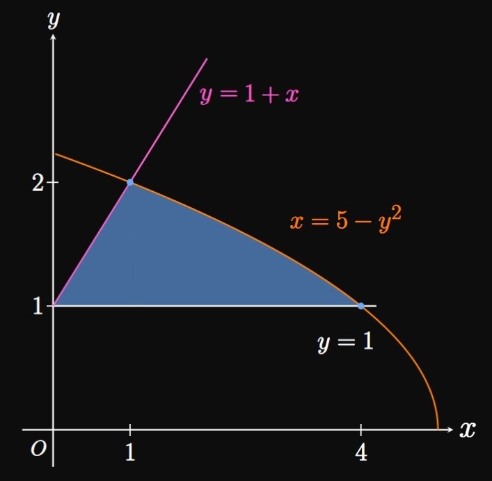
To sketch the curves, we note that \(x = 5 - y^2\) has a vertex at \((5, 0).\) As \(y\) increases, the graph arches through the first quadrant and hits the \(y\)-axis sometime after \(y = 2.\) To find when \(y = 1 + x\) intersects \(x = 5 - y^2,\) we express both functions in terms of one common variable. For example, we rearrange the former equation to get \(x = y - 1;\) then we find \[ \ba y - 1 &= 5 - y^2 \nl y^2 + y - 6 &= 0 \nl (y + 3)(y - 2) &= 0 \nl \implies y &= -3 \cma 2 \pd \ea \] Thus, in the first quadrant the line \(y = 1 + x\) crosses the parabola at \((1, 2).\) The line \(y = 1\) hits the parabola at the point \((4, 1).\) We therefore obtain the sketch in Figure 10.
Integrating with \(y\) It is easiest to integrate with \(y\) because for all \(y\) in the region, the function \(x = 5 - y^2\) is to the right of the line \(y = 1 + x.\) This means that the boundaries of the region remain the same. We therefore commit to integrating with \(y,\) so we must express all functions and bounds using \(y.\) We write the latter equation as \(x = y - 1.\) The region goes from \(y = 1\) to \(y = 2;\) thus, \(\eqrefer{eq:area-y}\) gives \[ \ba A &= \int_1^2 \parbr{(5 - y^2) - (y - 1)} \di y \nl &= \int_1^2 \par{6 - y - y^2} \di y \nl &= \par{6y - \tfrac{1}{2} y^2 - \tfrac{1}{3} y^3} \intEval_1^2 \nl &= \parbr{6(2) - \tfrac{1}{2}(2)^2 - \tfrac{1}{3}(2)^3} - \parbr{6(1) - \tfrac{1}{2}(1)^2 - \tfrac{1}{3}(1)^3} \nl &= \boxed{\tfrac{13}{6}} \ea \]
Integrating with \(x\) For \(0 \leq x \leq 1,\) the region's upper boundary is \(y = 1 + x\) and its lower boundary is \(y = 1.\) But for \(1 \leq x \leq 4,\) the upper boundary changes to \(x = 5 - y^2.\) Since these boundary functions are different, we must split the region at \(x = 1\) and add the areas of each region. Using \(\eqref{eq:area-x},\) the area of the left region is given by \[\int_0^1 \parbr{(1 + x) - 1} \di x \pd\] To find the area to the right of \(x = 1,\) we rewrite \(x = 5 - y^2\) as \(y = \sqrt{5 - x}.\) We then have \[\int_1^4 \par{\sqrt{5 - x} - 1} \di x \pd\] So the total area is \[A = \int_0^1 \parbr{(1 + x) - 1} \di x + \int_1^4 \par{\sqrt{5 - x} - 1} \di x \pd\] This integral setup also delivers the answer \(A = \boxed{13/6}.\)
We obtain the sketch in Figure 11. The parabola intersects \(x = 2 - y\) at \((1, 1)\) and crosses \(y = 4\) at \((2, 4).\) We now decide whether to cut the region vertically (integrating with \(x\)) or horizontally (integrating with \(y\)). In either case, we need to split the region and express all equations in terms of the respective variable.
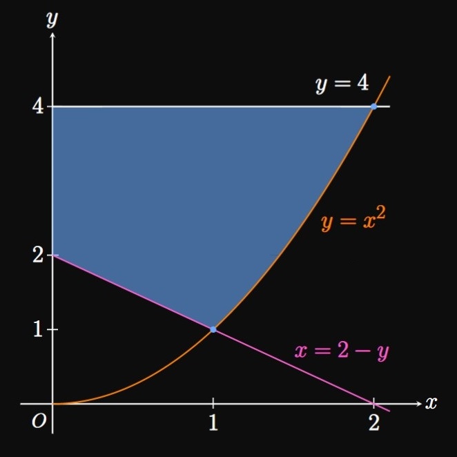
Integrating with \(x\) For \(0 \leq x \leq 1,\) the upper boundary is \(y = 4\) and the lower boundary is \(x = 2 - y.\) Yet for \(1 \leq x \leq 2,\) the upper boundary is \(y = 4\) but the lower boundary is \(y = x^2.\) Thus, we divide the region at \(x = 1\) and use \(\eqref{eq:area-x}\) to calculate the area of each subregion. Our next goal is to express all equations in terms of \(x.\) Solving for \(y\) in \(x = 2 - y\) gives \(y = 2 - x.\) Our area is therefore the sum \[A = \int_0^1 \parbr{4 - (2 - x)} \di x + \int_1^2 \par{4 - x^2} \di x \pd\]
Integrating with \(y\) If we integrate horizontally, then we need to be aware of any shifts in the region's boundaries. The shaded region for \(1 \leq y \leq 2\) is bounded right by \(y = x^2\) and left by \(x = 2 - y.\) But for \(2 \leq y \leq 4,\) the right boundary is \(y = x^2\) and the left boundary changes to the line \(x = 0.\) Thus, we split the region at \(y = 2\) and take the area of each subregion. Solving for \(x\) in \(y = x^2\) yields \(x = \sqrt y.\) Then using \(\eqref{eq:area-y}\) for each, we get \[A = \int_1^2 \parbr{\sqrt y - (2 - y)} \di y + \int_2^4 \par{\sqrt y - 0} \di y \pd \]
Either integral setup yields the answer of \(A = \boxed{25/6}.\) Thus, identify your options when choosing to integrate. When integrating with either \(x\) or \(y\) is convenient, be creative and use the method with which you feel most comfortable.
Areas with \(x\)
If \(f\) and \(g\) are continuous functions with \(f(x) \geq g(x)\) for \(a \leq x \leq b,\)
then the area bounded by \(y = f(x),\) \(y = g(x),\) the line \(x = a,\)
and the line \(x = b\) is
\[A = \int_a^b [f(x) - g(x)] \di x \pd \tag*{\(\eqref{eq:area-x}\)}\]
The geometric interpretation of this form is top function minus bottom function.
Areas with \(y\)
If \(f\) and \(g\) are continuous functions with \(f(y) \geq g(y)\) for \(c \leq y \leq d,\)
then the area bounded by \(x = f(y),\) \(x = g(y),\) the line \(y = c,\)
and the line \(y = d\) is
\[A = \int_c^d [f(y) - g(y)] \di y \pd \tag*{\(\eqref{eq:area-y}\)}\]
In this form, we integrate right function minus left function.
Problem-Solving Tips When calculating the area between curves, be flexible and select a method of integration. Use the following steps:
- Sketch the graphs and the region they enclose.
- Identify any points at which the boundary equations shift, and split the region at these points. Commit to integrating with respect to \(x\) or \(y\) and express all equations in terms of that variable.
- Find the intersection points of the graphs.
- Use \(\eqref{eq:area-x}\) for integration with \(x\) and \(\eqref{eq:area-y}\) for integration with \(y.\)