4.5: Numerical Integration

In Section 4.3 we learned a vital fact: the Fundamental Theorem of Calculus enables us to compute a definite integral \(\int_a^b f(x) \di x\) if we can find an antiderivative of \(f.\) Sadly, most functions have non-elementary antiderivatives, which can't be expressed using any combination of functions we know (such as polynomial, rational, radical, exponential, trigonometric, and logarithmic functions). For example, the functions \[\andThree{e^{x^2}}{\frac{1}{\sqrt{x^7 + 1}}}{\cos \par{x^2}}\] don't have elementary antiderivatives. To evaluate definite integrals with these functions, we must settle for an approximation if we work by hand. But understanding numerical integration allows us to write computer programs that can evaluate definite integrals almost exactly. These principles are based on the following topics:

• Endpoint Approximations
• Midpoint Rule
• Trapezoidal Rule
• Simpson's Rule

Endpoint Approximations

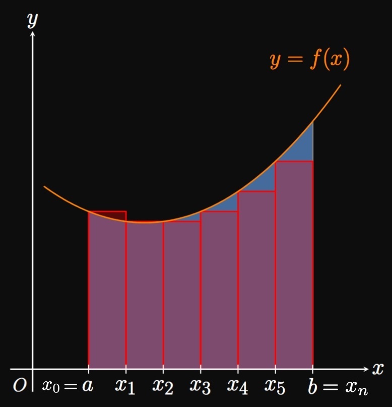
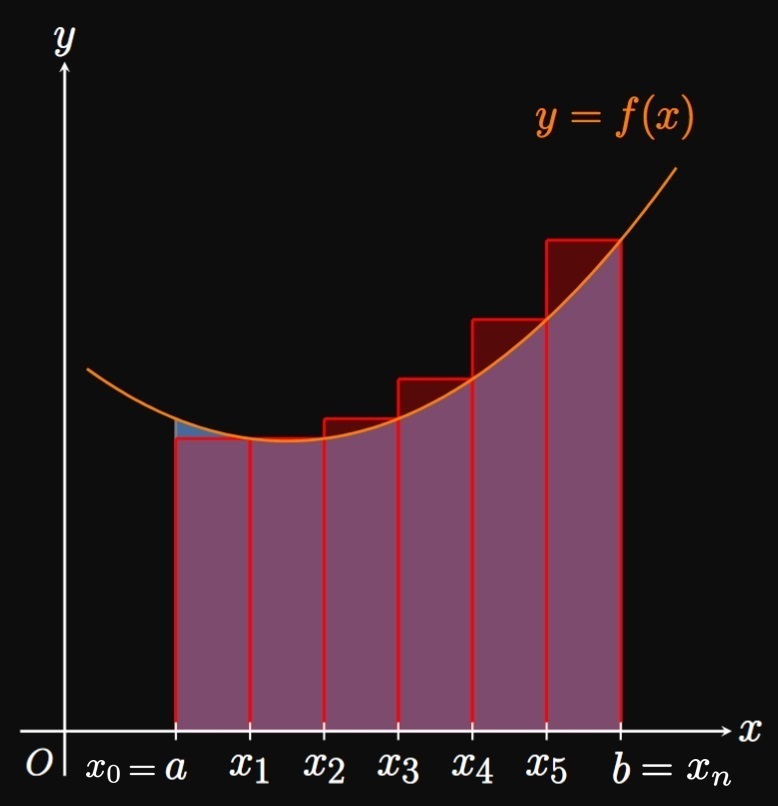
The simplest approximations to definite integrals use Riemann sums, in which we inscribe rectangles within a curve and add their areas. To estimate \(\int_a^b f(x) \di x,\) we first divide \([a, b]\) into \(n\) subintervals of endpoints \(a = x_0,\) \(x_1, \dots,\) \(x_{n - 1}, x_n = b\) and equal width \(\Delta x.\) In the general subinterval \(\parbr{x_{i - 1}, x_i},\) we evaluate \(f\) at a sample point \(x_i^*.\) An approximating rectangle in this subinterval has area \(f(x_i^*) \Delta x.\) We then sum the areas of all \(n\) rectangles, as we discussed in Section 4.2. In a left Riemann sum, we take \(x_i^* = x_{i - 1}\) and attain the approximation \begin{equation} \int_a^b f(x) \di x \approx L_n = \sum_{i = 1}^n f(x_{i - 1}) \Delta x \pd \label{eq:L-n} \end{equation} (See Figure 1A.) Likewise, a right Riemann sum uses \(x_i^* = x_i\) and provides the estimate \begin{equation} \int_a^b f(x) \di x \approx R_n = \sum_{i = 1}^n f(x_i) \Delta x \pd \label{eq:R-n} \end{equation} (See Figure 1B.) We call \(L_n\) and \(R_n\) the left-endpoint approximation and right-endpoint approximation, respectively.

Errors When we estimate a definite integral, our approximation will be wrong by some amount—called the error. For example, the error in the left-endpoint approximation is \[E_n = \underbrace{\int_a^b f(x) \di x}_{\text{true value}} - \underbrace{L_n}_{\text{our estimate}}\] and the error in the right-endpoint approximation is \[E_n = \underbrace{\int_a^b f(x) \di x}_{\text{true value}} - \underbrace{R_n}_{\text{our estimate}} \pd\] Unless we know the exact value of \(\int_a^b f(x) \di x\) (if so, then why even approximate?), we cannot find the exact error \(E_n.\) Instead, we can find an error bound—a number whose magnitude is greater than or equal to the magnitude of the error. It turns out that endpoint approximations to \(\int_a^b f(x) \di x\) have an error bound given by \begin{equation} \abs{E_n} \leq \frac{M_1 (b - a)^2}{2n} \cma \label{eq:E-bound-endpts} \end{equation} where \(\abs{f'(x)} \leq M_1\) on \([a, b].\) Simply put, when we use \(\eqref{eq:L-n}\) or \(\eqref{eq:R-n}\) to approximate \(\int_a^b f(x) \di x,\) we can be sure our estimate is off by no more than the prescribed magnitude in \(\eqref{eq:E-bound-endpts}.\) As we increase \(n\)—that is, as we inscribe more, thinner rectangles within a curve—our approximation grows in accuracy. So it's intuitive that the error bound in \(\eqref{eq:E-bound-endpts}\) decreases with \(n.\) Unfortunately, the proofs of all the error bounds in this section are beyond the scope of this text.

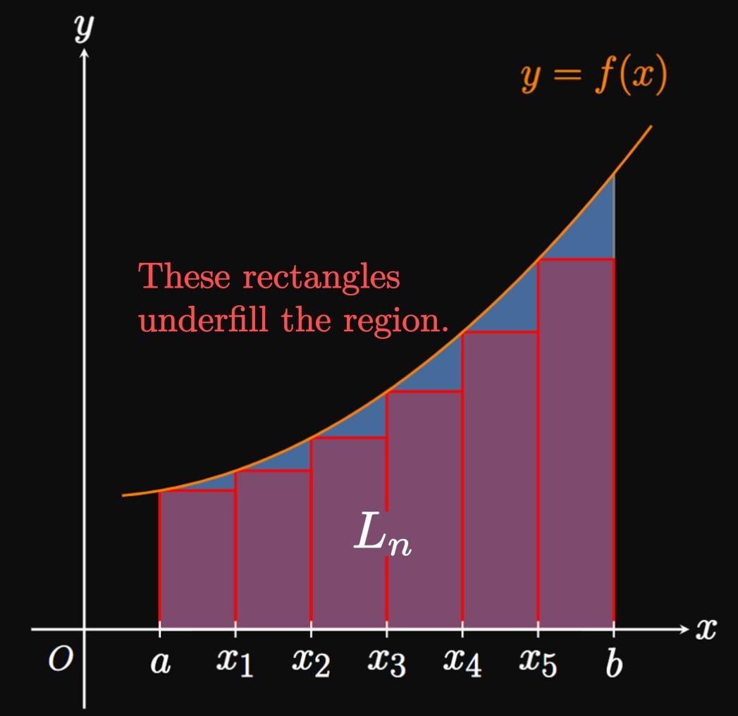
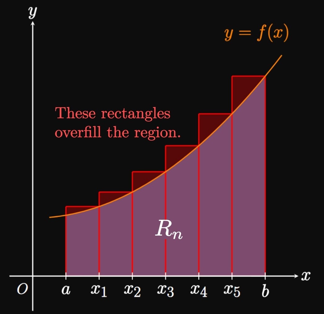
If \(f\) is increasing on \([a, b],\) then a left-endpoint approximation underestimates \(\int_a^b f(x) \di x\) and a right-endpoint approximation overestimates \(\int_a^b f(x) \di x.\) For the particular case \(f(x) \geq 0,\) the rectangles positioned at the left endpoints miss portions of the bounded region (Figure 2A), whereas rectangles positioned at the right endpoints capture excess area (Figure 2B). Mathematically, we say \[L_n \leq \int_a^b f(x) \di x \leq R_n \pd\] Conversely, if \(f\) is decreasing on \([a, b],\) then a left-endpoint approximation overestimates \(\int_a^b f(x) \di x\) and a right-endpoint approximation underestimates \(\int_a^b f(x) \di x.\) Symbolically, we have \[R_n \leq \int_a^b f(x) \di x \leq L_n \pd\] (By sketching a positive decreasing curve, you may verify that a left Riemann sum overfills a region and a right Riemann sum underfills the region.)

We estimate the area using four approximating rectangles of equal width \(\Delta x = 2/4\) \(= 0.5.\) Using \(\eqref{eq:R-n}\) with \(f(x) = x^2\) and \(n = 4,\) we estimate \(\int_0^2 x^2 \di x\) to be \[ \ba R_4 &= \sum_{i = 1}^4 x_i^2 \Delta x \nl &= \parbr{(0.5)^2 + (1)^2 + (1.5)^2 + (2)^2} (0.5) \nl &= \boxed{3.75} \ea \]

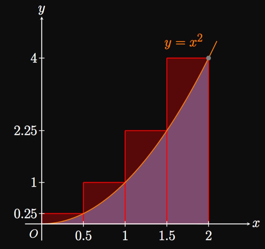
Error Because \(f(x) = x^2\) is increasing on \(0 \leq x \leq 2,\) the right-endpoint approximation is an overestimate, as shown by the excess area in Figure 3. Observe that \(f'(x) = 2x,\) whose maximum on \([0, 2]\) is \(4.\) Hence, we use \(\eqref{eq:E-bound-endpts}\) with \(M_1 = 4\) and \(n = 4\) to get an error bound of \[ \abs{E_4} \leq \frac{4 (2 - 0)^2}{2(4)} = \boxed 2 \]

The error bound of \(\abs{E_4} \leq 2\) in Example 1 guarantees that the approximation \(R_4 = 3.75\) differs from the true value of \(\int_0^2 x^2 \di x\) by no more than \(2.\) Yet the integral happens to be easy to evaluate; by the Fundamental Theorem of Calculus, \[\int_0^2 x^2 \di x = \tfrac{1}{3} x^3 \intEval_0^2 = \tfrac{8}{3} \approx 2.667 \pd\] Hence, our right-endpoint approximation indeed overestimated this value by roughly \(1.083,\) so the error in the estimate was \(-1.083,\) whose magnitude is within \(2.\) But most definite integrals cannot be calculated exactly; we deliberately chose the simple example \(\int_0^2 x^2 \di x\) to illustrate the concept of error.

Midpoint Rule

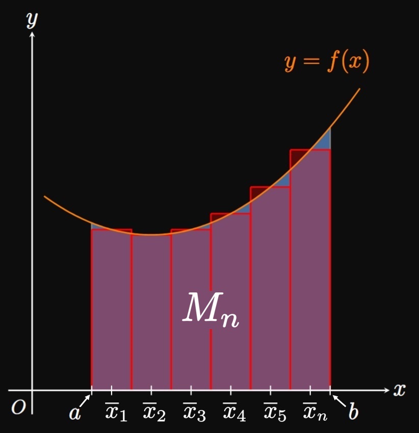
Instead of taking the sampling point \(x_i^*\) to be an endpoint of \(\parbr{x_{i - 1}, x_i},\) we can let \(x_i^*\) be the midpoint \[\overline x_i = \tfrac{1}{2} (x_{i - 1} + x_i) \pd\] This method leads to the Midpoint Rule, in which we use the approximation \begin{equation} \int_a^b f(x) \di x \approx M_n = \sum_{i = 1}^n f(\overline x_i) \Delta x \pd \label{eq:M-n} \end{equation} (See Figure 4.) The error bound for the Midpoint Rule is \begin{equation} \abs{E_M} \leq \frac{M_2 (b - a)^3}{24n^2} \cma \label{eq:E-M} \end{equation} where \(\abs{f''(x)} \leq M_2\) on \([a, b].\) In general, the Midpoint Rule is more accurate than Endpoint Approximations because rectangles positioned at the midpoints \(\overline x_1,\) \(\overline x_2,\) \(\dots, \overline x_n\) are more effective in capturing a bounded region.

Geometrically, we construct five rectangles of equal width \(\Delta x = (4 - 1)/5\) \(= 0.6\) and sum their areas. The subintervals are \([1, 1.6],\) \([1.6, 2.2],\) \([2.2, 2.8],\) \([2.8, 3.4],\) and \([3.4, 4];\) we sample the midpoint of each subinterval. (See Figure 5.) The Midpoint Rule, as in \(\eqref{eq:M-n},\) therefore estimates \(\int_1^4 (1/x) \di x\) to be \[ \ba M_5 &= \sum_{i = 1}^5 \frac{1}{\overline x_i} \Delta x \nl &= \par{\frac{1}{1.3} + \frac{1}{1.9} + \frac{1}{2.5} + \frac{1}{3.1} + \frac{1}{3.7}} (0.6) \nl &\approx \boxed{1.373} \ea \] If \(f(x) = 1/x,\) then \(f'(x) = -1/x^2\) and \(f''(x) = 2/x^3.\) The maximum value of \(\abs{f''(x)}\) over \([1, 4]\) is \(\abs{f''(1)} = 2.\) So in \(\eqref{eq:E-M}\) we substitute \(M_2 = 2\) and \(n = 5\) to find \[ \abs{E_M} \leq \frac{2 (4 - 1)^3}{24(5)^2} = \boxed{0.09} \] Thus, our estimation of \(M_5 = 1.373\) differs from the true value of \(\int_1^4 (1/x) \di x\) by no more than \(0.09.\)

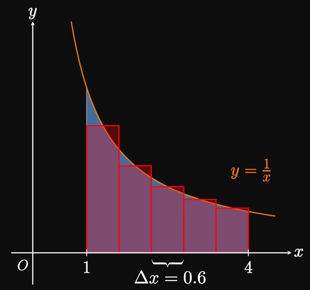
Again, we intentionally chose an integral in Example 2 whose exact value is easily determined. By the Fundamental Theorem of Calculus, we see \[\int_1^4 \frac{1}{x} \di x = \ln \abs x \intEval_1^4 = \ln 4 \approx 1.386 \pd\] Our estimate of \(M_5 = 1.373\) was very close! On the other hand, endpoint approximations would give \(L_5 \approx 1.638\) and \(R_5 \approx 1.188.\) By comparing values, we see that the Midpoint Rule tends to be more accurate than endpoint approximations.

Trapezoidal Rule

Instead of using rectangles, we could use trapezoids to estimate an integral. In the general subinterval \(\parbr{x_{i - 1}, x_i},\) we construct a trapezoid of heights \(f(x_{i - 1})\) and \(f(x_i)\) and width \(\Delta x,\) as shown by Figure 6. Recall that a trapezoid of heights \(h_1\) and \(h_2\) and width \(w\) has area \(A = \tfrac{1}{2} (h_1 + h_2) w.\) Taking the width of all the approximating trapezoids to be \(\Delta x,\) we sum their areas to attain \begin{align} \int_a^b f(x) \di x &\approx T_n \nonum \nl &= \tfrac{1}{2} [f(x_0) + f(x_1)] \Delta x + \tfrac{1}{2} [f(x_1) + f(x_2)] \Delta x + \cdots + \tfrac{1}{2} \parbr{f(x_{n - 1}) + f(x_n)} \Delta x \nonum \nl &= \frac{\Delta x}{2} \parbr{f(x_0) + 2 f(x_1) + 2f(x_2) + \cdots + 2 f(x_{n - 1}) + f(x_n)} \pd \label{eq:T-n} \end{align} This approximation, called the Trapezoidal Rule, is the average of the left-endpoint approximation and right-endpoint approximation; namely, \(T_n = \tfrac{1}{2} (L_n + R_n).\) We derived the Trapezoidal Rule for positive functions, but it works for any continuous function \(f.\) The error in a trapezoidal approximation satisfies \begin{equation} \abs{E_T} \leq \frac{M_2 (b - a)^3}{12 n^2} \cma \label{eq:E-T} \end{equation} where \(\abs{f''(x)} \leq M_2\) for \(a \leq x \leq b.\) Because the Trapezoidal Rule and Midpoint Rule each account for a graph's curvature, they are usually more accurate than endpoint approximations. Note that error bounds for the Trapezoidal Rule and Midpoint Rule depend on \(\abs{f''(x)},\) while the error bound for endpoint approximations depends on \(\abs{f'(x)}.\)

We inscribe five trapezoids (of equal width) under the curve \(y = 1/x\) and sum their areas. (See Figure 7.) Observe that \(\Delta x = (4 - 1)/5\) \(= 0.6.\) So our subintervals are \([1, 1.6],\) \([1.6, 2.2],\) \([2.2, 2.8],\) \([2.8, 3.4],\) and \([3.4, 4].\) We therefore use the Trapezoidal Rule in \(\eqref{eq:T-n}\) to approximate the integral as \[ \ba T_5 &= \frac{0.6}{2} \parbr{\frac{1}{1} + 2 \par{\frac{1}{1.6}} + 2 \par{\frac{1}{2.2}} + 2 \par{\frac{1}{2.8}} + 2 \par{\frac{1}{3.4}} + \par{\frac{1}{4}}} \nl &\approx \boxed{1.413} \ea \] If \(f(x) = 1/x,\) then the maximum of \(\abs{f''(x)} = 2/x^3\) on \([1, 4]\) is \(\abs{f''(1)} = 2.\) The error bound is, following \(\eqref{eq:E-T}\) with \(M_2 = 2\) and \(n = 5,\) \[\abs{E_5} \leq \frac{2 (4 - 1)^3}{12 (5)^2} = \boxed{0.18}\] Compare \(T_5 = 1.413\) to the result of Example 2, which gave a more accurate approximation for \(\int_1^4 (1/x) \di x.\)

Simpson's Rule

When we use the Trapezoidal Rule, we approximate the area under a positive function \(f\) by constructing lines—that is, using first-degree polynomials—and taking the areas under the lines. Now let's extend this idea by using second-degree polynomials, quadratics. Let's first develop a useful formula: We will fit a quadratic \(y = Ax^2 + Bx + C\) through three points with equal horizontal spacing; let's call them \((x_0, y_0),\) \((x_1, y_1),\) and \((x_2, y_2),\) where \(x_1 = \tfrac{1}{2} (x_0 + x_2)\) and \[ \ba y_1 &= A x_1^2 + B x_1 + C \nl &= A \par{\frac{x_0 + x_2}{2}}^2 + B \par{\frac{x_0 + x_2}{2}} + C \pd \ea \] Our goal is to use these \(y\)-values to find an expression for \(\int_{x_0}^{x_2} p(x) \di x\) (the area under the parabola, in the special case where \(y_0,\) \(y_1,\) and \(y_2\) are positive). We see \[ \ba \int_{x_0}^{x_2} \par{Ax^2 + Bx + C} \di x &= \frac{A \par{x_2^3 - x_0^3}}{3} + \frac{B \par{x_2^2 - x_0^2}}{2} + C(x_2 - x_0) \nl &= \frac{x_2 - x_0}{6} \parbr{2A \par{x_0^2 + x_0x_2 + x_2^2} + 3B(x_2 + x_0) + 6 C} \pd \ea \] Through expansion and collecting terms, we see that the expression in brackets is \[\underbrace{\par{Ax_0^2 + B x_0 + C}}_{y_0} + \underbrace{4 \parbr{A \par{\frac{x_0 + x_2}{2}}^2 + B \par{\frac{x_0 + x_2}{2}} + C}}_{4 y_1} + \underbrace{\par{Ax_2^2 + B x_2 + C}}_{y_2} \pd\] Hence, we have \begin{equation} \int_{x_0}^{x_2} \par{Ax^2 + Bx + C} \di x = \frac{x_2 - x_0}{6} \par{y_0 + 4 y_1 + y_2} \pd \label{eq:parabola-integral} \end{equation}

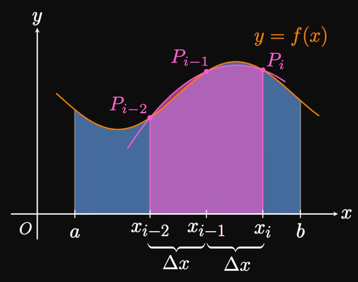
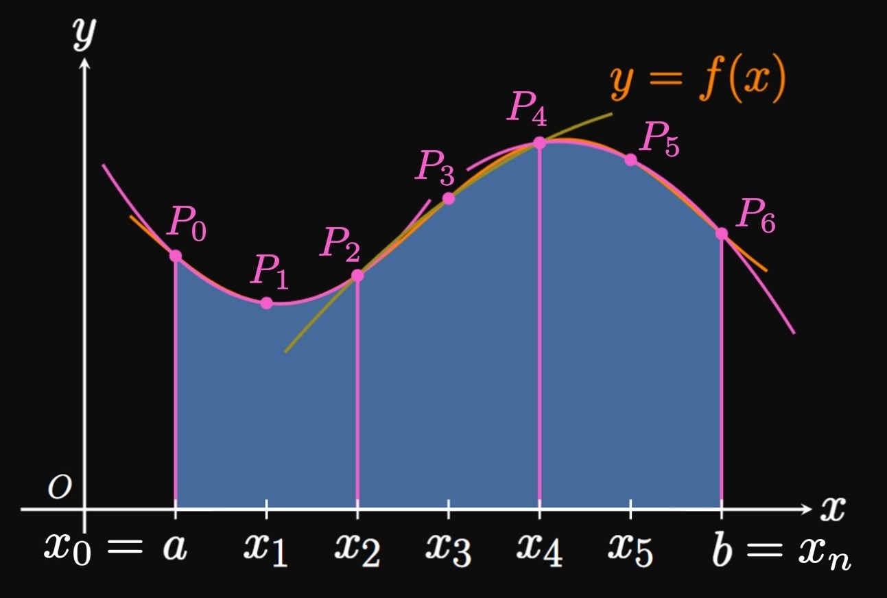
Now we return to our question—how do we approximate a definite integral \(\int_a^b f(x) \di x\) using parabolas? We first cut \([a, b]\) into \(n\) subintervals with endpoints \(a = x_0, x_1, \dots,\) \(x_n = b\) and equal width \(\Delta x.\) But this time \(n\) must be even. In the general double subinterval \(\parbr{x_{i - 2}, x_i},\) we construct a parabola that passes through the points \(P_{i - 2} \par{x_{i - 2}, f(x_{i - 2})},\) \(P_{i - 1} \par{x_{i - 1}, f(x_{i - 1})},\) and \(P_i \par{x_i, f(x_i)}.\) In the special case where \(f(x) \geq 0,\) the area under the parabola approximates the area under \(f\) on \(\parbr{x_{i - 2}, x_i},\) as shown by Figure 8. Now if we decrease \(\Delta x,\) then the points \(P_{i - 2},\) \(P_{i - 1},\) and \(P_i\) become closer to each other; accordingly, the parabola better follows the shape of \(f.\) In fact, as \(\Delta x \to 0,\) the parabola becomes indistinguishable from \(f\) on \(\parbr{x_{i - 2}, x_i},\) so the area under the parabola becomes closer to the exact area under \(f.\) (See Animation 1.) Hence, we approximate the area under \(f\) on \(\parbr{x_{i - 2}, x_i}\) to be, following \(\eqref{eq:parabola-integral},\) \[\frac{2 \Delta x}{6} \parbr{f(x_{i - 2}) + 4 f(x_{i - 1}) + f(x_i)} = \frac{\Delta x}{3} \parbr{f(x_{i - 2}) + 4 f(x_{i - 1}) + f(x_i)} \pd\] If we repeat this argument for all subintervals in \([a, b],\) as in Figure 9, then we attain the following approximation for \(\int_a^b f(x) \di x \col\) \begin{align} S_n &= \small \frac{\Delta x}{3} \parbr{f(x_0) + 4 f(x_1) + f(x_2)} + \frac{\Delta x}{3} \parbr{f(x_2) + 4 f(x_3) + f(x_4)} + \cdots + \frac{\Delta x}{3} \parbr{f(x_{n - 2}) + 4 f(x_{n - 1}) + f(x_n)} \nonum \nl &= \small \frac{\Delta x}{3} \parbr{f(x_0) + 4 f(x_1) + 2 f(x_2) + 4 f(x_3) + \cdots + 2 f(x_{n - 2}) + 4 f(x_{n - 1}) + f(x_n)} \pd \label{eq:simpson} \end{align} This approximation is called Simpson's Rule. Observe that the coefficients follow the pattern \(1, 4, 2, 4, 2, 4,\) \(\dots, 4, 2, 4, 1.\) Although we derived this rule for positive functions, it works equally as well for any continuous function \(f.\) As \(n \to \infty,\) Simpson's Rule gives the exact value of \(\int_a^b f(x) \di x.\) So as we construct approximations, we remember that larger values of \(n\) provide better estimates.

The error bound in Simpson's Rule depends on the fourth derivative of \(f.\) If \(\abs{f^{(4)}(x)} \leq M_4\) for \(a \leq x \leq b,\) then the error \(E_S\) satisfies \begin{equation} \abs{E_S} \leq \frac{M_4 (b - a)^5}{180 n^4} \pd \label{eq:E-S} \end{equation} Let's summarize the main differences in the error bounds for all the numerical integration methods in this section:

• The error bound for an endpoint approximation depends on \(\abs{f'(x)}.\)
• The error bound for the Midpoint Rule or Trapezoidal Rule depends on \(\abs{f''(x)}.\)
• The error bound for Simpson's Rule depends on \(\abs{f^{(4)}(x)}.\)

If we repeat Example 5 with \(n = 10,\) then we get the estimate \(S_{10} = 0.85563.\) Likewise, using \(n = 20\) gives \(S_{20} = 0.85562.\) These approximations are close to exact value of \(\int_0^1 e^{-x^2/2} \di x.\) In a computer program, in which \(n\) can be as large as \(400,\) definite integrals can therefore be calculated accurately to several decimal places. (You can write a program to run the Midpoint Rule, the Trapezoidal Rule, or Simpson's Rule using only a few lines of code.)