1.4: Continuity
In everyday language, the word continuous might describe a phenomenon that occurs without interruption. But in mathematics, we require a description to have a clear, standard definition. So in this section we provide a formal definition of continuity, explore its uses, and learn to classify discontinuities. We discuss the following topics:
- Continuity at a Point
- Continuity over an Interval
- Continuity of Combinations of Functions
- Intermediate Value Theorem
Continuity at a Point
Informally, we say a function \(f\) is continuous at \(a\)
if we can trace the curve \(y = f(x)\)
near \(x = a\) without lifting our pen.
Simply put, \(f\) is continuous at \(a\) if the graph does not have a break
at \(x = a.\)
But formally, we define \(f\) to be continuous at \(a\) if and only if
\begin{equation}
\lim_{x \to a} f(x) = f(a) \pd \label{eq:cont-point}
\end{equation}
This definition requires us to check three conditions:
- \(f(a)\) is defined.
- \(\ds \lim_{x \to a} f(x)\) exists.
- \(\ds \lim_{x \to a} f(x)\) equals \(f(a).\)
Many phenomena are continuous: A plant's height changes continuously with time because its height doesn't increase abruptly. Likewise, a car's position is a continuous function of time since the car can't teleport. And the volume of a leaking container decreases continuously due to the laws of physics.

It's easy to identify discontinuities on a graph, but how do we detect them from equations? Let's classify the three types of discontinuities—removable discontinuities, jump discontinuities, and infinite discontinuities.
Removable Discontinuities A function \(f(x)\) has a removable discontinuity (also called a hole) at \(x = a\) if \(\lim_{x \to a} f(x)\) exists but does not equal \(f(a).\) Alternatively, \(f(a)\) may be undefined. In Figure 1, the graph of \(y = f(x)\) has a removable discontinuity at \(x = a\) because \[\lim_{x \to a} f(x) = K \ne f(a) \pd\] We call this discontinuity removable because we may fill in the hole at \((a, K)\) to restore continuity. By doing so, we construct a new function \(g\) that matches \(f\) but is continuous at \(a\)—namely, \[g(x) = \begin{cases} f(x) &x \ne a \nl K &x = a \pd \end{cases} \]
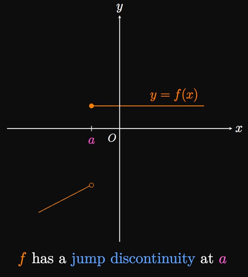
Jump Discontinuities The function \(f(x)\) has a jump discontinuity at \(x = a\) if the one-sided limits \[\lim_{x \to a^-} f(x) \and \lim_{x \to a^+} f(x)\] exist but don't equal each other. (See Figure 2.) The name is self-explanatory: at \(x = a,\) an abrupt jump interrupts the graph of \(f.\)
Infinite Discontinuities Lastly, the function \(f(x)\) has an infinite discontinuity at \(x = a\) if either \[\lim_{x \to a^-} f(x) \or \lim_{x \to a^+} f(x)\] is infinite. At \(x = a,\) the graph of \(y = f(x)\) has a vertical asymptote; \(f\) is therefore unbounded near the line \(x = a.\) (See Figure 3.)

- \(f(x)\) has a removable discontinuity at \(x = a\) if \(\lim_{x \to a} f(x)\) exists but does not equal \(f(a).\)
- \(f(x)\) has a jump discontinuity at \(x = a\) if the one-sided limits \[\lim_{x \to a^-} f(x) \and \lim_{x \to a^+} f(x)\] exist and do not equal each other.
- \(f(x)\) has an infinite discontinuity at \(x = a\) if either \[\lim_{x \to a^-} f(x) \or \lim_{x \to a^+} f(x)\] is infinite.
One-Sided Continuity How do we discuss continuity at endpoints? To do so, we establish the following definitions: \(f\) is continuous from the left at \(a\) if and only if \[\lim_{x \to a^-} f(x) = f(a) \pd\] Likewise, \(f\) is continuous from the right at \(a\) if and only if \[\lim_{x \to a^+} f(x) = f(a) \pd\] As we communicate mathematical ideas, we must be able to describe a graph's behavior in great detail; these definitions facilitate this goal.
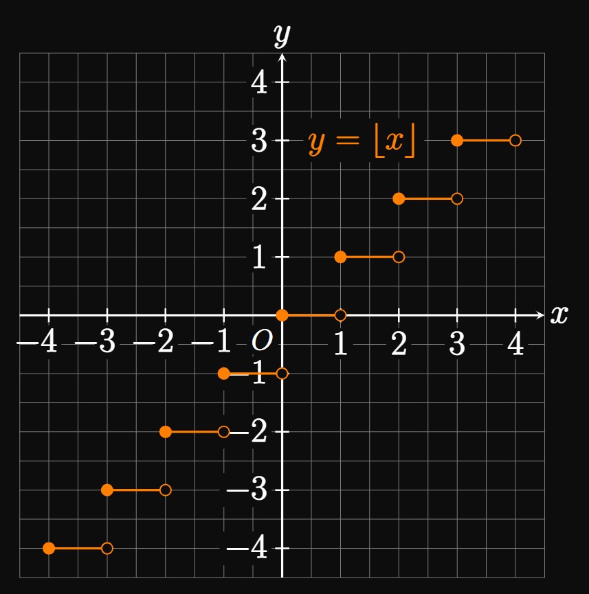
Greatest Integer Function
The greatest-integer function \(y = \floor x\) returns
the greatest integer equal to or less than \(x.\)
Figure 4 shows the graph of this function,
which has jump discontinuities at all integers \(n.\)
(For example, the greatest integer function has a jump discontinuity
at the integer \(1\) since \(\lim_{x \to 1^-} \floor x = 0\)
but \(\lim_{x \to 1^+} \floor x\)
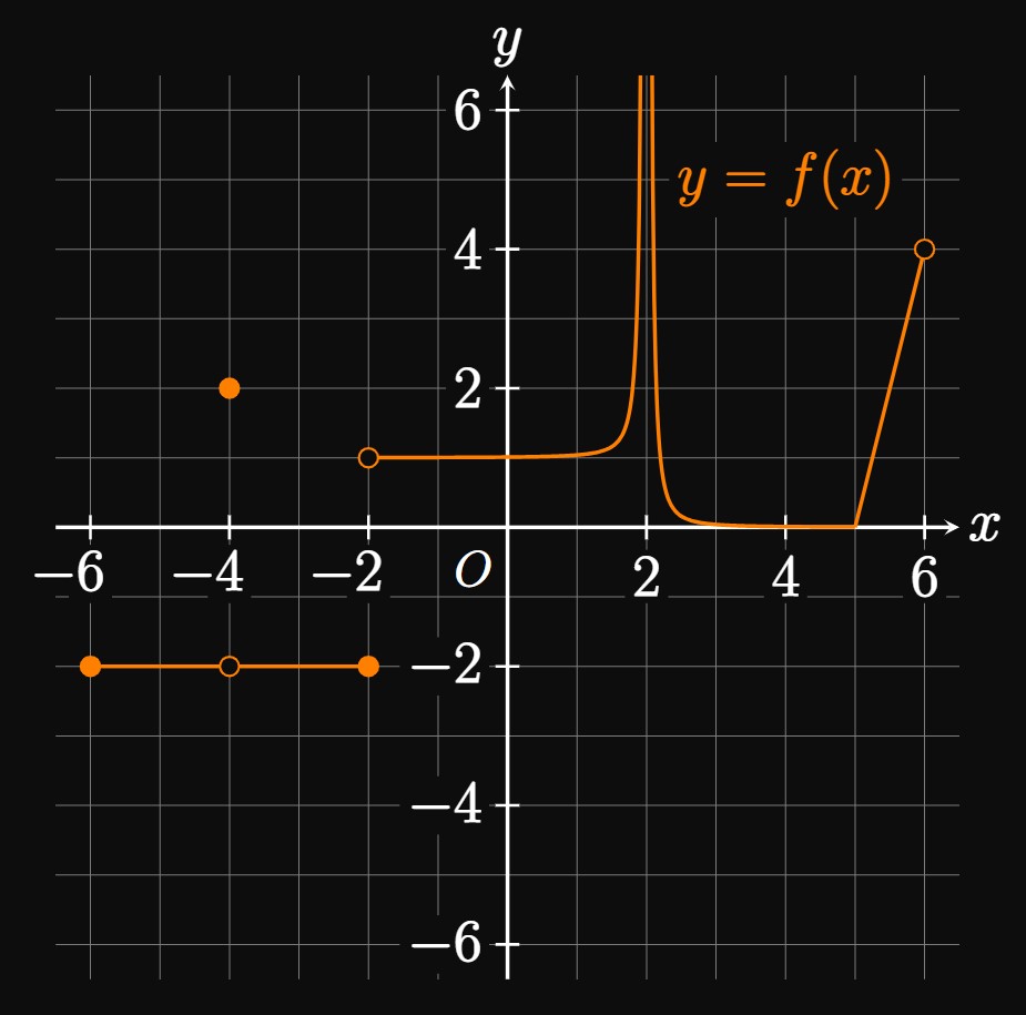
The function \(f\) has a removable discontinuity at \(x = -4,\) a jump discontinuity at \(x = -2,\) and an infinite discontinuity at \(x = 2.\) Also, \(f\) is continuous from the right at \(x = -6\) because \[\lim_{x \to -6^+} f(x) = f(-6) = -2 \pd \] Yet \(f\) is discontinuous at \(x = 6\) since \(f(6)\) does not exist.
- \(\ds f(x) = \frac{x^2 - 16}{x + 4} \cmaa x = -4\)
- \(\ds f(x) = \frac{1}{x + 3} \cmaa x = -3 \)
- \(\ds f(x) = \bc x - 2 &x \lt 2 \nl 3(3 - x)^2 &x \geq 2 \cmaa \ec x = 2 \)
- The numerator of \(f(x)\) is a difference of squares: \[x^2 - 16 = (x + 4)(x - 4) \pd\] We therefore see \[ \ba \lim_{x \to -4} f(x) &= \lim_{x \to -4} \frac{\cancel{(x + 4)}(x - 4)}{\cancel{x + 4}} \nl &= \lim_{x \to -4} (x - 4) = -8 \pd \ea \] Thus, \[\lim_{x \to -4^-} f(x) = \lim_{x \to -4^+} f(x) = -8 \pd\] Since both one-sided limits at \(-4\) equal each other [but \(f(-4)\) is undefined], \(f(x)\) has a removable discontinuity at \(x = -4.\)
- The graph of \(y = 1/(x + 3)\) has a vertical asymptote at \(x = -3\) because \[\lim_{x \to -3^-} f(x) = -\infty \and \lim_{x \to -3^+} f(x) = \infty \pd\] Therefore, \(f\) has an infinite discontinuity at \(-3.\)
- We see \[ \baat{2} \lim_{x \to 2^-} f(x) &= 2 - 2 &&= 0 \cma \nl \lim_{x \to 2^+} f(x) &= 3(3 - 2)^2 &&= 3 \pd \eaat \] Since these one-sided limits exist but don't equal each other, \(f\) has a jump discontinuity at \(2.\)
Continuity over an Interval
Figure 6A shows the graph of \(y = f(x)\) over the open interval \(a \lt x \lt b.\) We say \(f\) is continuous over the open interval \((a, b)\) because \[\lim_{x \to c} f(x) = f(c)\] is satisfied by all \(c\) in \((a, b).\) Conversely, Figure 6B shows the graph of \(y = f(x)\) over the closed interval \(a \leq x \leq b.\) We see \(f(x)\) is continuous from the right at \(x = a\) because \[\lim_{x \to a^+} f(x) = f(a) \pd\] Likewise, \(f(x)\) is continuous from the left at \(x = b\) since \[\lim_{x \to b^-} f(x) = f(b) \pd\] Hence, a function \(f\) is said to be continuous over a closed interval \([a, b]\) if and only if the following statements are true:
- \(f\) is continuous over the open interval \((a, b).\)
- \(\ds \lim_{x \to a^+} f(x) = f(a)\) and \(\ds \lim_{x \to b^-} f(x) = f(b).\)
We say a function \(f\) is continuous if it is continuous at each point in its domain. Many functions are continuous on their domains. For example, polynomials are continuous for all real numbers, and logarithms are continuous for strictly positive inputs. The following table provides the intervals of continuity for many functions we've seen: polynomial, rational, radical, absolute value, exponential, logarithmic, trigonometric, and inverse trigonometric.
| Function | Interval of Continuity |
|---|---|
| Polynomials: \(c_n x^n + c_{n - 1} x^{n - 1} + \cdots + c_1 x + c_0\) | \(-\infty \lt x \lt \infty\) |
| Rational expressions: \(P(x)/Q(x),\) where \(P\) and \(Q\) are polynomials | All \(x\) such that \(Q(x) \ne 0\) |
| \(\sin x\) | \(-\infty \lt x \lt \infty\) |
| \(\cos x\) | \(-\infty \lt x \lt \infty\) |
| \(\tan x\) | \(\ds x \ne \frac{\pi}{2} \pm n \pi\) |
| \(\csc x\) | \(\ds x \ne \pm n \pi\) |
| \(\sec x\) | \(\ds x \ne \frac{\pi}{2} \pm n \pi\) |
| \(\cot x\) | \(\ds x \ne \pm n \pi\) |
| \(b^x \cma b \gt 0\) | \(-\infty \lt x \lt \infty\) |
| \(\log_b x \cma b \gt 0\) and \(b \ne 1\) | \(x \gt 0\) |
| \(\sqrt[n]{x} \cma n\) odd | \(-\infty \lt x \lt \infty\) |
| \(\sqrt[n] x \cma n\) even | \(x \geq 0\) |
| \(\abs x\) | \(-\infty \lt x \lt \infty\) |
| \(\sin^{-1} x\) | \(-1 \leq x \leq 1\) |
| \(\cos^{-1} x\) | \(-1 \leq x \leq 1\) |
| \(\tan^{-1} x\) | \(-\infty \lt x \lt \infty\) |
In Section 1.2 we introduced the method of evaluating limits by Direct Substitution. The preceding table enables us to extend this method to nearly every function.
Continuity of Combinations of Functions
Let's discuss the continuity of sums, differences, products, and quotients of functions.
If \(f\) and \(g\) are each continuous at \(a,\)
then \((f + g),\) \((f - g),\) \((f \cdot g),\)
and [assuming \(g(a)\)
- \(f(x) + g(x)\)
- \(f(x) - g(x)\)
- \(f(x) \cdot g(x)\)
- \(f(x)/g(x) \cmaa\) \(\; g(a) \ne 0.\)
Continuity of Composite Functions A composite function is of the form \(f(g(x)).\) If this function is continuous at \(a,\) then we have \begin{equation} \lim_{x \to a} f(g(x)) = f(g(a)) \pd \label{eq:comp-funct-continuous} \end{equation} In using \(\eqref{eq:comp-funct-continuous},\) we require \(g\) to be continuous at \(a\) and \(f\) to be continuous at \(g(a).\) Then the composite function is continuous at \(a.\)
PROOF Let \(L = g(a).\) If \(g\) is continuous at \(a,\) then \(\lim_{x \to a} g(x) = L.\) In Section 1.3 we learned to evaluate the limit of a composite function as follows: \[\lim_{x \to a} f(g(x)) = \lim_{t \to L} f(t) \pd\] Since \(f\) is continuous at \(L = g(a),\) we have \[\lim_{t \to L} f(t) = f(L) = f(g(a)) \cma\] thus giving \(\eqref{eq:comp-funct-continuous}.\) \[\qedproof\]
Intermediate Value Theorem
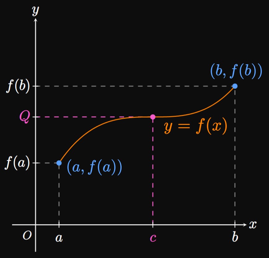
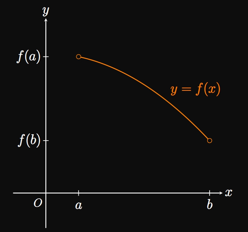
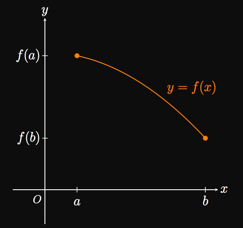
Continuity provides us an important application, the Intermediate Value Theorem: If \(f\) is continuous on \([a, b],\) then \(f\) takes on every value between \(f(a)\) and \(f(b).\) Intuitively, a continuous curve that begins at \((a, f(a))\) and ends at \((b, f(b))\) must contain any intermediate point that lies between these endpoints. To express this idea mathematically, we let \(Q\) be any intermediate value between \(f(a)\) and \(f(b)\)–that is, \(f(a) \leq Q \leq f(b).\) Then the Intermediate Value Theorem guarantees the existence of some \(c\) in \([a, b]\) for which \(f(c) = Q.\) (See Figure 7.) Some functions have multiple values of \(c\) in \([a, b]\) that satisfy the Intermediate Value Theorem; these functions take on the value \(Q\) multiple times in \([a, b].\) But the Intermediate Value Theorem does not give us a method to find \(c;\) it merely proves the existence of such \(c.\)
The proof of the Intermediate Value Theorem relies on deeper properties of the real number system, typically studied in a real analysis course, and is therefore omitted here.

Graphing Calculators
Example 10
shows how graphing calculators find zeros:
The graphing calculator plots two points with opposite \(y\)-values,
assumes the function is continuous,
and connects the points.
An algorithm enables the calculator to sample many points
to attain an accurate guess of the zero.
For example, we could use the Intermediate Value Theorem again in
Example 10
by noting that \(f(0.2) = -1.18272\) and \(f(0.8) = 0.53472,\)
so the zero \(c\) must lie in \((0.2, 0.8).\)
As we repeat this process with \(f(0.5) = -1.125\)
and \(f(0.75) = 0.04296875,\)
the Intermediate Value Theorem again asserts that the zero \(c\)
must lie in \((0.5, 0.75).\)
We can continue sampling points to attain a narrower
interval, thus approaching the true value of \(c.\)
A computer can iterate this operation many times to get
a zero that is accurate to many decimal places.
(It turns out that \(c \approx\)
Continuity at a Point The function \(f(x)\) is continuous at \(x = a\) if and only if \begin{equation} \lim_{x \to a} f(x) = f(a) \pd \eqlabel{eq:cont-point} \end{equation} This definition requires three conditions:
- \(f(a)\) is defined.
- \(\ds \lim_{x \to a} f(x)\) exists.
- \(\ds \lim_{x \to a} f(x)\) equals \(f(a).\)
If any of these conditions is false, then \(f\) is discontinuous at \(a.\) We classify discontinuities using three categories:
- \(f(x)\) has a removable discontinuity at \(x = a\) if \(\lim_{x \to a} f(x)\) exists but does not equal \(f(a).\)
- \(f(x)\) has a jump discontinuity at \(x = a\) if the one-sided limits \[\lim_{x \to a^-} f(x) \and \lim_{x \to a^+} f(x)\] both equal different numbers.
- \(f(x)\) has an infinite discontinuity at \(x = a\) if either \[\lim_{x \to a^-} f(x) \or \lim_{x \to a^+} f(x)\] is infinite.
We also discuss one-sided continuity as follows: The function \(f\) is continuous from the left at \(a\) if and only if \[\lim_{x \to a^-} f(x) = f(a)\] and is continuous from the right at \(a\) if and only if \[\lim_{x \to a^+} f(x) = f(a) \pd\]
Continuity over an Interval If a function \(f(x)\) is continuous at every point in \((a, b),\) continuous from the right at \(x = a,\) and continuous from the left at \(x = b,\) then \(f(x)\) is continuous over \([a, b].\) Many functions are continuous on their domains; the following table shows the intervals over which some functions are continuous. Let \(n\) be a positive integer.
| Function | Interval of Continuity |
|---|---|
| Polynomials: \(c_n x^n + c_{n - 1} x^{n - 1} + \cdots + c_1 x + c_0\) | \(-\infty \lt x \lt \infty\) |
| Rational expressions: \(P(x)/Q(x),\) where \(P\) and \(Q\) are polynomials | All \(x\) such that \(Q(x) \ne 0\) |
| \(\sin x\) | \(-\infty \lt x \lt \infty\) |
| \(\cos x\) | \(-\infty \lt x \lt \infty\) |
| \(\tan x\) | \(\ds x \ne \frac{\pi}{2} \pm n \pi\) |
| \(\csc x\) | \(\ds x \ne \pm n \pi\) |
| \(\sec x\) | \(\ds x \ne \frac{\pi}{2} \pm n \pi\) |
| \(\cot x\) | \(\ds x \ne \pm n \pi\) |
| \(b^x \cma b \gt 0\) | \(-\infty \lt x \lt \infty\) |
| \(\log_b x \cma b \gt 0\) and \(b \ne 1\) | \(x \gt 0\) |
| \(\sqrt[n]{x} \cma n\) odd | \(-\infty \lt x \lt \infty\) |
| \(\sqrt[n] x \cma n\) even | \(x \geq 0\) |
| \(\abs x\) | \(-\infty \lt x \lt \infty\) |
| \(\sin^{-1} x\) | \(-1 \leq x \leq 1\) |
| \(\cos^{-1} x\) | \(-1 \leq x \leq 1\) |
| \(\tan^{-1} x\) | \(-\infty \lt x \lt \infty\) |
Continuity of Combinations of Functions If \(f(x)\) and \(g(x)\) are both continuous at \(x = a,\) then the following combinations of \(f(x)\) and \(g(x)\) are also continuous at \(x = a \col\)
- \(f(x) + g(x)\)
- \(f(x) - g(x)\)
- \(f(x) \cdot g(x)\)
- \(f(x)/g(x) \cmaa\) \(\; g(a) \ne 0.\)
If \(g(x)\) is continuous at \(x = a\) and \(f(x)\) is continuous at \(x = g(a),\) then \(f(g(x))\) is continuous at \(x = a;\) namely, \begin{equation} \lim_{x \to a} f(g(x)) = f(g(a)) \pd \eqlabel{eq:comp-funct-continuous} \end{equation}
Intermediate Value Theorem If \(f\) is continuous on \([a, b],\) and \(Q\) is a number between \(f(a)\) and \(f(b),\) then the Intermediate Value Theorem guarantees a value \(c\) in \([a, b]\) such that \(f(c) = Q.\) In other words, the theorem says that on \([a, b],\) the continuous function \(f\) takes on every value between \(f(a)\) and \(f(b).\)