Chapter 8: Differential Equations
In Section 4.1 we learned the basics of differential equations. Differential equations relate a function to its rates of change; in many scenarios, it is far easier to model the rate of change. In this chapter we learn techniques for solving differential equations. But when differential equations have no analytical solutions, numerical approximations and geometric blueprints (8.1) become critical. We will learn several applications of differential equations, such as mixing solute in a tank, orthogonal trajectories, population growth, objects cooling down, capacitors discharging, analyzing chemical reactions, and disease spread—all by writing and solving differential equations.
Sections
8.1 Slope Fields and Euler's Method
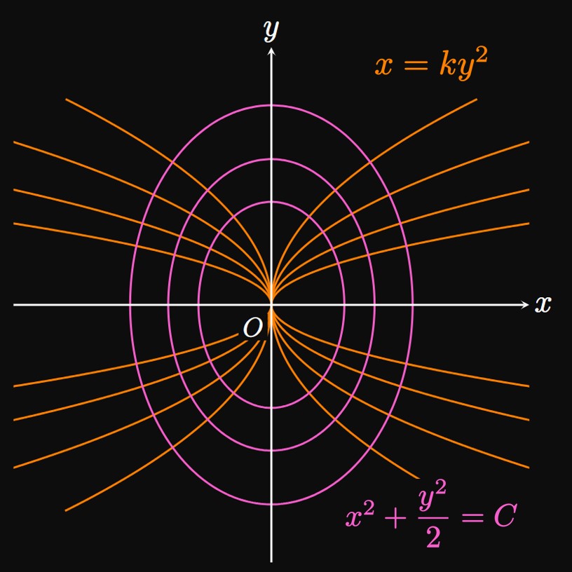
Defining a differential equation and verifying solutions to differential equations. Euler's Method to approximate solutions to differential equations. Sketching and interpreting slope fields. Solving a first-order differential equation by separating variables, with mathematical proof. Particular solutions to initial value problems. Mixing problems and orthogonal trajectories. Modeling with exponential growth and decay. Doubling time and half-life. Compound interest, Newton's Law of Cooling, unrestricted population growth, discharging a capacitor, and first-order chemical reactions.8.4 Logistic Models
Controlled growth and decay through the logistic function. Properties of logistic functions. Applications to population growth, disease spread, and social media activity. Solving first-order linear equations of the form \(y' + P(x)y = Q(x)\) using integrating factors.