0.9: Exponents and Logarithms

Many operations in mathematics rely on exponents and logarithms. Understanding these topics is crucial for engaging with calculus. In this section we review the following topics:

Exponents and Exponential Functions
Logarithms and Logarithmic Functions

Exponents and Exponential Functions

In an exponential function, the exponent is a variable. An example is \(f(x) = 2^x,\) whereas \(g(x) = x^2\) is a power function since the base is a variable. In general, an exponential function is of the form \begin{equation} f(x) = b^x \label{eq:def-exp} \end{equation} where \(b\) is a positive constant with \(b \ne 1.\)

What does the power of an exponential function really mean? Let's take \(n\) to be any positive integer. In \(\eqref{eq:def-exp}\) the simplest case is \(x = n,\) which represents repeated multiplication: \[b^n = \underbrace{b \cdot b \cdot \, \cdots \, \cdot b}_{n \text{ factors}} \pd\] But if \(x = -n\) then \[b^{-n} = \frac{1}{b^n} = \frac{1}{\underbrace{b \cdot b \cdot \, \cdots \, \cdot b}_{n \text{ factors}}} \pd\] Recall that any nonzero number raised to the power of \(0\) equals \(1;\) that is, \(b^0 = 1.\) If \(x\) is a rational number, \(x = p/q,\) where \(p\) and \(q\) are positive integers, then \[b^x = b^{p/q} = \sqrt[q]{b^p} \pd\] To evaluate \(\sqrt[q]{b^p},\) we first raise \(b\) to the power of \(p\) and then take the \(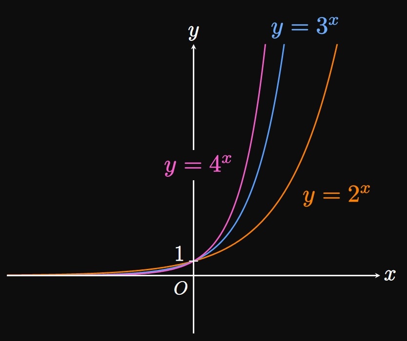q \,\)th root; for example, \[\sqrt[3]{8^2} = \sqrt[3]{64} = 4 \pd\]

The preceding interpretations enable us to sketch the graphs of exponential functions. Figure 1A shows the graphs of \(y = 2^x,\) \(y = 3^x,\) and \(y = 4^x.\) Exponential functions with larger bases grow more rapidly. In addition, since \((1/b)^x\) \(= b^{-x},\) the graph of \(y = (1/b)^x\) is the reflection of \(y = b^x\) across the \(y\)-axis: Figure 1B shows the graphs of \(y = (1/2)^x,\) \(y = (1/3)^x,\) and \(y = (1/4)^x.\) The graph of \(y = (1/b)^x,\) \(b \gt 1,\) is therefore said to exhibit exponential decay. Note that all exponential graphs have a \(y\)-intercept of \((0, 1)\) because \(b^0 = 1.\) These functions also have a domain of \((-\infty, \infty)\) and a range of \((0, \infty).\)

EXAMPLE 1

Sketch the graph of \(y = 5 - 3^x.\) Identify the domain and range.

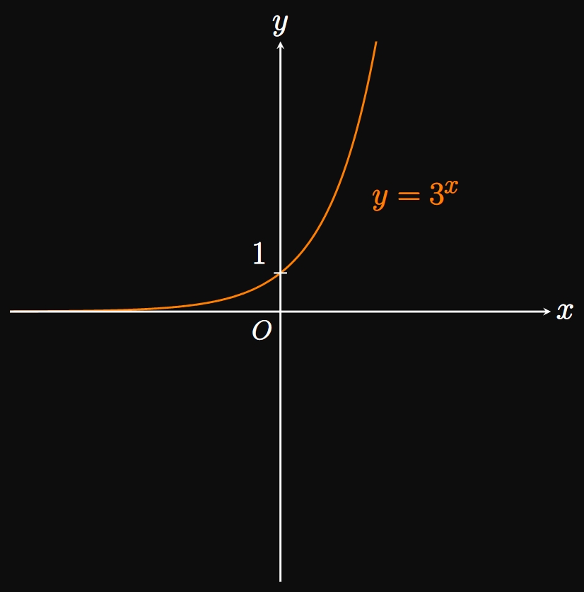
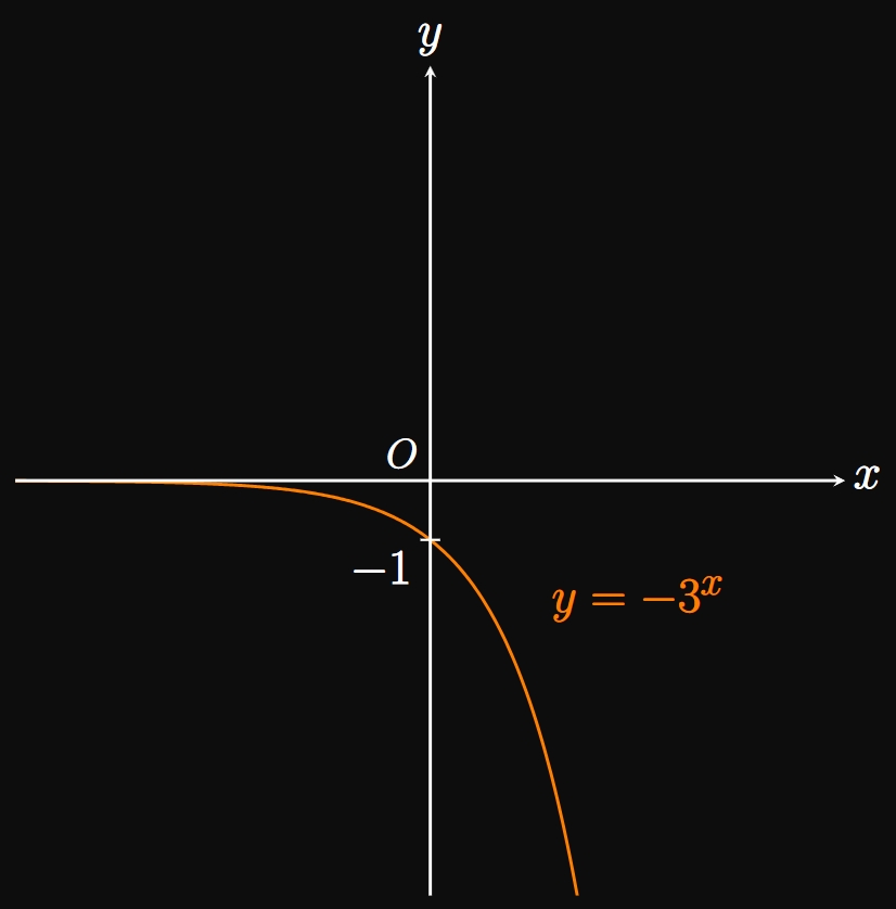
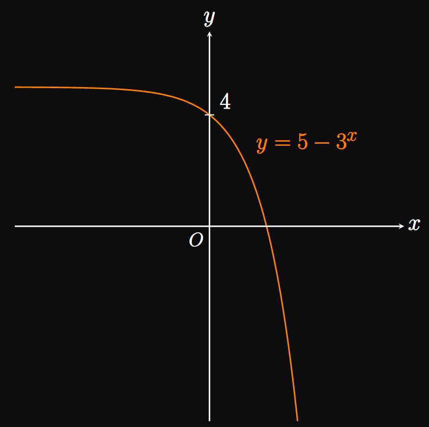
First we sketch the parent graph of \(y = 3^x,\) as shown in Figure 2A. Then we reflect the graph across the \(x\)-axis (Figure 2B) and finally translate it \(5\) units upward (Figure 3). The domain is \((-\infty, \infty),\) and the range is \((-\infty, 5).\)

Next we discuss rules with exponents, shown below. Although we omit the proofs of these properties, we encourage you to experiment with numbers and verify that they are true.

LAWS OF EXPONENTS

Let \(a\) and \(b\) be positive numbers, and let \(m\) and \(n\) be any real numbers. Then the exponent laws are as follows: \begin{align} a^{m + n} &= a^m \, a^n \cma \label{eq:exp-law-add} \nl a^{m - n} &= \frac{a^m}{a^n} \cma \label{eq:exp-law-minus} \nl \par{a^{m}}^n &= a^{mn} \cma \label{eq:exp-law-mn} \nl \par{ab}^n &= a^n \, b^n \pd \label{eq:exp-law-a-b} \end{align}

EXAMPLE 2

If \(w,\) \(x,\) and \(y\) are nonzero numbers and \(x\) is positive, then simplify \[\frac{\par{4 w^2 \, x^3 \sqrt[3]{y}}^3}{\par{2 w^4 \, y^2 \sqrt x}^2} \pd\]

Note that \(\sqrt[3] y\) \(= y^{1/3}\) and \(\sqrt x\) \(= x^{1/2}.\) We therefore use exponent properties as follows: \[ \baat{2} \frac{\par{4 w^2 \, x^3 \sqrt[3]{y}}^3}{\par{2 w^4 \, y^2 \sqrt x}^2} &= \frac{\par{4 w^2 \, x^3 \, y^{1/3}}^3}{\par{2 w^4 \, y^2 \, x^{1/2}}^2} \nl &= \frac{(4)^3 \par{w^2}^3 \par{x^3}^3 \par{y^{1/3}}^3}{(2)^2 \par{w^4}^2 \par{y^2}^2 \par{x^{1/2}}^2} \comment{\text{by } \eqref{eq:exp-law-a-b}} \nl &= \frac{64 w^6 \, x^9 \, y}{4 w^8 \, y^4 \, x} \comment{\text{by } \eqref{eq:exp-law-mn}} \nl &= \boxed{\frac{16 x^8}{w^2 \, y^3}} \comment{\text{by } \eqref{eq:exp-law-minus}} \eaat \]

EXAMPLE 3

Solve for \(x\) in the equation \[2^{x + 1} = 8^{3x - 1} \pd\]

We can't equate the powers, as the bases are different. But we can equate the powers if the bases are the same, so let's force both sides to have the same base. Noting that \(8 = 2^3,\) we rewrite the equation as \[ \ba 2^{x + 1} &= \par{2^3}^{3x - 1} \nl 2^{x + 1} &= 2^{9x - 3} \cma \ea \] where the last step is true by \(\eqref{eq:exp-law-mn}.\) Since the bases are the same, we equate the exponents to get \[ \ba x + 1 &= 9x - 3 \nl \implies x &= \boxed{\tfrac{1}{2}} \ea \]

Logarithms and Logarithmic Functions

If \(b \gt 0\) and \(b \ne 1,\) then the exponential function \(f(x) = b^x\) is either increasing or decreasing. Accordingly, the graph is one-to-one; it passes the Horizontal Line Test. Then \(f\) has an inverse function called the logarithmic function, \(\inv f(x) = \log_b x.\) Exponents and logarithms therefore share the following bidirectional relationship: \begin{equation} y = b^x \iffArrow x = \log_b y \pd \label{eq:exp-log} \end{equation} So a logarithmic function of base \(b,\) when given a number \(y,\) outputs the power to which \(b\) must be raised to give \(y.\) For example, \(2^3 = 8\) implies \(\log_2 8 = 3\) because \(2\) must be raised to the power of \(3\) to become \(8.\) Likewise, since \(b^1 = b\) and \(b^0 = 1,\) it follows that \begin{equation} \log_b b = 1 \and \log_b 1 = 0 \pd \label{eq:log-1} \end{equation}

Special Logarithms The common logarithm is a logarithm of base \(10.\) In this text, the common logarithm is written simply as \(\log\) with no base, so \(\log x\) strictly means \(\log_{10} x.\) For example, \(\log 100 = 2\) since \(10^2 = 100.\) Ironically, in calculus the common logarithm is used far less than the natural logarithm, whose base is Euler's number—the irrational number \(e \approx 2.718.\) The natural logarithm is denoted as \(\ln;\) for example, \(\ln \par{e^2} = 2\) because \(2\) is the power to which \(e\) must be raised to attain \(e^2.\) Euler's number satisfies many beautiful mathematical properties, and we will formally define it in Chapter 2.

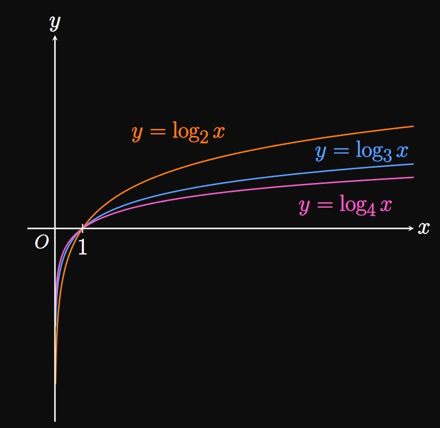
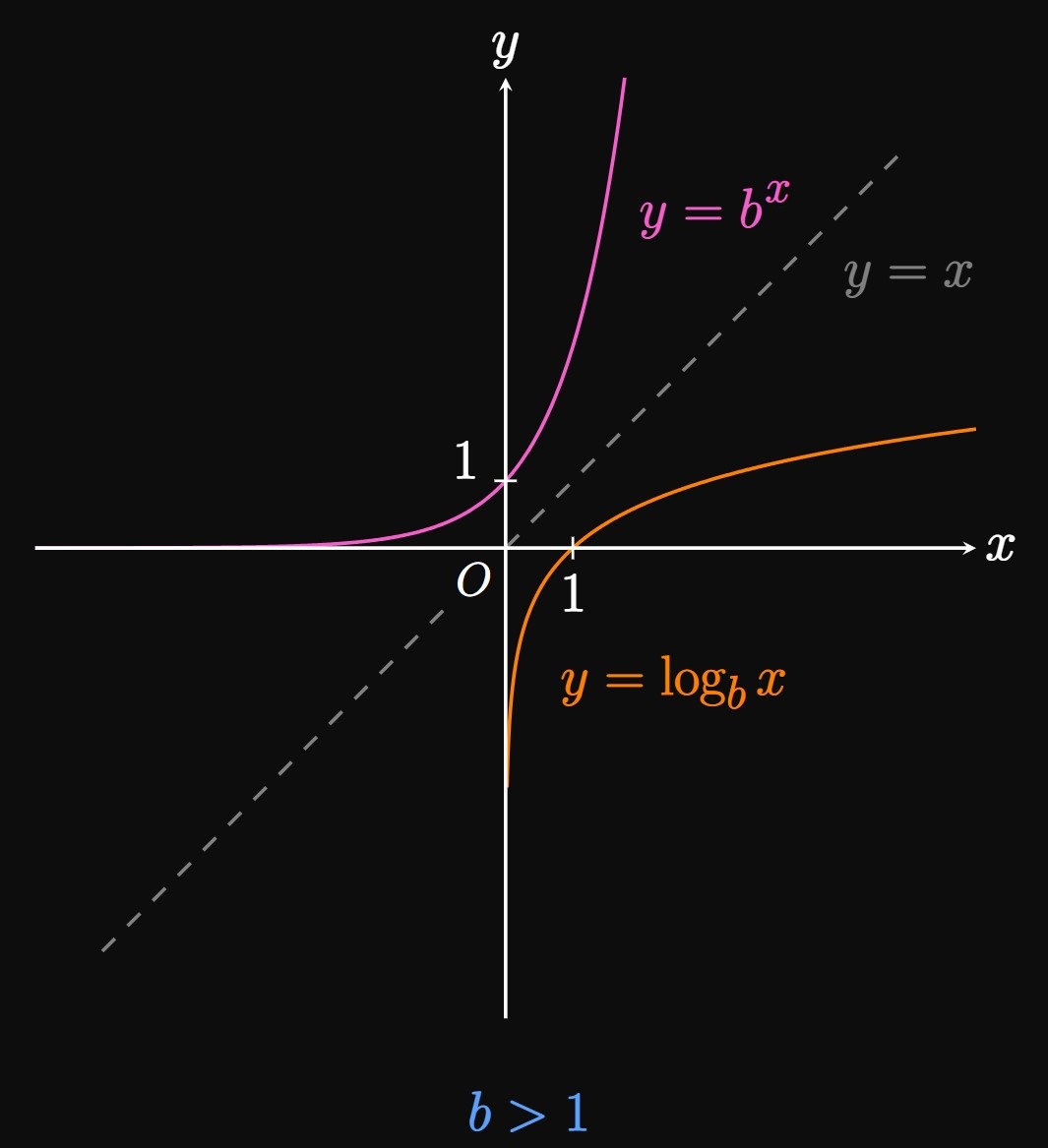
Because the exponential function and the logarithmic function are inverses of each other, their graphs are reflections of each other across the line \(y = x.\) Because \(y = b^x\) passes through \((0, 1),\) \(y = \log_b x\) passes through \((1, 0).\) Most useful logarithms have bases greater than \(1,\) so let's consider \(b \gt 1.\) Then the graph of \(y = \log_b x\) is shown by Figure 4. Whereas \(y = b^x\) increases rapidly, \(y = \log_b x\) grows painfully slowly. Examine that \(\log 100\) \(= 2,\) \(\log 1000\) \(= 3,\) and \(\log 10000\) \(= 4.\) Figure 5 shows the graphs of \(y = \log_2 x,\) \(y = \log_3 x,\) and \(y = \log_4 x.\) All of these graphs have an \(x\)-intercept of \((1, 0),\) a domain of \((0, \infty),\) and a range of \((-\infty, \infty).\)

EXAMPLE 4

Evaluate the following logarithms.

\(\log_3 81\)
\(\log_4 2\)
\(\log_8 \frac{1}{64}\)

Let's use \(\eqref{eq:exp-log}\) to help us interpret each logarithmic expression.

Since \(3^4 = 81,\) the logarithm gives the power: \[\log_3 81 = \boxed 4\]

Taking the square root of \(4\)—that is, raising \(4\) to the power of \(1/2\)—gives \(2.\) Accordingly, \[\log_4 2 = \boxed{\tfrac{1}{2}}\]

Note that \(8^2 = 64,\) so \(8^{-2} = 1/64.\) The logarithm equals the power: \[\log_8 \tfrac{1}{64} = \boxed{-2}\]

EXAMPLE 5

Solve for \(x\) in the equation \[\tfrac{1}{3} \log_4 x + 7 = 8 \pd\]

It is a good idea to first isolate the logarithm, as follows: \[ \ba \tfrac{1}{3} \log_4 x &= 1 \nl \log_4 x &= 3 \pd \ea \] Then consulting \(\eqref{eq:exp-log}\) gives \[x = 4^3 = \boxed{64}\]

In Example 5, as we solve \(\log_4 x = 3,\) another perspective is to exponentiate both sides: \[ \ba \cancel{4}^{\cancel{\log_4} x} &= 4^3 \nl x &= 4^3 = 64 \pd \ea \] In general, for \(x \gt 0,\) \begin{equation} b^{\log_b x} = x \pd \label{eq:exp-log-cancel} \end{equation} Thus, by exponentiating both sides of an equation, we can strip logarithms.

The properties of logarithms are shown below, and the proofs for these rules are left as exercises.

LAWS OF LOGARITHMS

Let \(b\) be a positive number with \(b \ne 1.\) If \(x\) and \(y\) are positive numbers and \(p\) is any real number, then the logarithm laws are as follows: \begin{align} \log_b(xy) &= \log_b x + \log_b y \cma \label{eq:log-add} \nl \log_b \par{\frac{x}{y}} &= \log_b x - \log_b y \cma \label{eq:log-minus} \nl \log_b \par{x^p} &= p \log_b x \pd \label{eq:log-p} \end{align}

In words, logarithms enable us to split a product into a sum [by \(\eqref{eq:log-add}\)] and a quotient into a difference [by \(\eqref{eq:log-minus}\)]. \(\eqrefer{eq:log-p}\) asserts that any power inside a logarithm can be pulled to the front.

EXAMPLE 6

Expand the following logarithm: \[\log_5 \par{\frac{25 a^3 \, b^7}{\sqrt c}} \cma\] where \(a,\) \(b,\) and \(c\) are positive.

The word expand tells us to break the logarithm into several terms. Noting that \(\sqrt c\) \(= c^{1/2},\) we have \[ \baat{2} \log_5 \par{\frac{25 a^3 \, b^7}{\sqrt c}} &= \log_5 \par{\frac{25 a^3 \, b^7}{c^{1/2}}} \nl &= \log_5 \par{25 a^3 \, b^7} - \log_5 \par{c^{1/2}} \comment{\text{by } \eqref{eq:log-minus}} \nl &= \log_5 25 + \log_5 \par{a^3} + \log_5 \par{b^7} - \log_5 \par{c^{1/2}} \comment{\text{by } \eqref{eq:log-add}} \nl &= 2 + \log_5 \par{a^3} + \log_5 \par{b^7} - \log_5 \par{c^{1/2}} \comment{\text{since } 5^2 = 25} \nl &= \boxed{2 + 3 \log_5 a + 7 \log_5 b - \tfrac{1}{2} \log_5 c} \comment{\text{by } \eqref{eq:log-p}} \eaat \]

EXAMPLE 7

Condense the following expression into a single logarithm: \[\tfrac{1}{2} \log x - 3 \log y + 4 \log z \cma\] where \(x,\) \(y,\) and \(z\) are positive.

Because each logarithm has the same base \((10),\) logarithm laws enable us to merge the logarithms: \[ \baat{2} \tfrac{1}{2} \log x - 3 \log y + 4 \log z &= \log \par{x^{1/2}} - \log \par{y^3} + \log \par{z^4} \comment{\text{by } \eqref{eq:log-p}} \nl &= \log \par{\frac{x^{1/2} \, z^4}{y^3}} \comment{\text{by } \eqref{eq:log-add} \text{ and } \eqref{eq:log-minus}} \nl &= \boxed{\log \par{\frac{\sqrt x \, z^4}{y^3}}} \eaat \]

Change of Base Formula Not all logarithms can be evaluated by hand, so a calculator may be necessary. But many scientific calculators only have one base for the logarithmic function, either log or ln. We therefore need a formula that enables us to convert between logarithmic bases. Letting \(y = \log_b x,\) where \(b\) is a positive number and \(b \ne 1,\) we have \(x = b^y\) by \(\eqref{eq:exp-log}.\) On both sides we take the logarithm of any base \(c\) \((c \gt 0\) and \(c \ne 1)\) and use \(\eqref{eq:log-p} \col\) \begin{align} \log_c x &= \log_c \par{b^y} \nonum \nl \log_c x &= y \log_c b \nonum \nl y &= \frac{\log_c x}{\log_c b} \nonum \nl \log_b x &= \frac{\log_c x}{\log_c b} \pd \label{eq:log-change-base} \end{align} This form enables us to compute logarithms on scientific calculators that offer only one base; as an example, \[\log_9 7 = \frac{\log 7}{\log 9} = \frac{\ln 7}{\ln 9} \approx 0.886 \pd\]

CHANGE OF BASE FORMULA FOR LOGARITHMS

If \(b\) and \(c\) are positive numbers such that \(b \ne 1\) and \(c \ne 1,\) then the Change of Base Formula for Logarithms gives \begin{equation} \log_b x = \frac{\log_c x}{\log_c b} \pd \eqlabel{eq:log-change-base} \end{equation}

EXAMPLE 8

Using a calculator, solve for \(x\) to three decimal places: \[4^{2x} = 5^{x - 1} \pd\]

Compare this problem to Example 3; there is no way to force \(4\) and \(5\) to have the same base. Instead, we take the logarithm of both sides and use \(\eqref{eq:log-p}.\) (The base to use is irrelevant; we just need to bring down the powers. Let's use the common logarithm.) Doing so, we get \[ \ba \log \par{4^{2x}} &= \log \par{5^{x - 1}} \nl 2x \log 4 &= (x - 1) \log 5 \nl 2x \log 4 &= x \log 5 - \log 5 \nl 2x \log 4 - x \log 5 &= - \log 5 \nl x (2 \log 4 - \log 5) &= - \log 5 \nl \implies x &= \frac{-\log 5}{2 \log 4 - \log 5} \pd \ea \] Evaluating \(\log 4\) and \(\log 5\) using a calculator, we attain \(\boxed{x \approx -1.384}.\)

EXAMPLE 9

Solve for \(x\) in the equation \[25^x - 5^x - 2 = 0 \pd\]

Note that \(25 = 5^2,\) so the equation becomes \[\par{5^x}^2 - 5^x - 2 = 0 \pd\] This equation resembles a quadratic equation for which factoring yields \[\par{5^x - 2} \par{5^x + 1} = 0 \pd\] Equating each factor to \(0,\) we get \[ \ba 5^x - 2 &= 0 \lspace &5^x + 1 &= 0 \nl 5^x &= 2 \lspace &5^x &= -1 \nl x &= \log_5 2 \pd \ea \] Note that \(5^x = -1\) has no solutions because \(5^x\) has a range of \((0, \infty).\) So the only solution is \(\boxed{x = \log_5 2} \approx 0.431.\)

EXAMPLE 10

Solve for \(x\) in the equation \[\log_6 x + \log_6 (x - 16) = 2 \pd\]

Note that the domain of \(\log_6 x\) \(+ \log_6 (x - 16)\) is \((16, \infty)\) (so that neither logarithm has a nonpositive input). We solve the equation as follows: \[ \baat{2} \log_6 (x^2 - 16x) &= 2 \comment{\text{by } \eqref{eq:log-add}} \nl x^2 - 16x &= 36 \comment{\text{by } \eqref{eq:exp-log}} \nl x^2 - 16x - 36 &= 0 \nl (x - 18)(x + 2) &= 0 \pd \eaat \] Equating each factor to \(0\) gives \(x = 18\) and \(x = -2.\) But \(x = -2\) is an extraneous solution because it is outside of the domain; instead, the only solution is \(\boxed{x = 18}.\)

Exponents and Exponential Functions In an exponential function, the power is a variable: \begin{equation} f(x) = b^x \eqlabel{eq:def-exp} \end{equation} where \(b\) is a positive constant with \(b \ne 1.\) If \(b \gt 1,\) then the graph of \(y = b^x\) exhibits exponential growth, growing rapidly. But the graph of \(y = (1/b)^x\) undergoes exponential decay and so decreases. An exponential graph has a \(y\)-intercept of \((0, 1),\) a domain of \((-\infty, \infty),\) and a range of \((0, \infty).\) Let \(a\) and \(b\) be positive numbers, and let \(m\) and \(n\) be any real numbers. Then the exponent laws are as follows: \begin{align} a^{m + n} &= a^m \, a^n \cma \eqlabel{eq:exp-law-add} \nl a^{m - n} &= \frac{a^m}{a^n} \cma \eqlabel{eq:exp-law-minus} \nl \par{a^{m}}^n &= a^{mn} \cma \eqlabel{eq:exp-law-mn} \nl \par{ab}^n &= a^n \, b^n \pd \eqlabel{eq:exp-law-a-b} \end{align}

Logarithms and Logarithmic Functions The logarithmic function \(\log_b x\) is the inverse function of the exponential function \(b^x.\) Exponents and logarithms therefore have the following bidirectional relationship: \begin{equation} y = b^x \iffArrow x = \log_b y \pd \eqlabel{eq:exp-log} \end{equation} In words, the logarithm gives the power \(x\) to which \(b\) must be raised to produce \(y.\) Given that \(b^1 = b\) and \(b^0 = 1,\) examples of logarithm applications are \begin{equation} \log_b b = 1 \and \log_b 1 = 0 \pd \eqlabel{eq:log-1} \end{equation} In addition, exponentiating a logarithmic expression cancels the logarithm: \begin{equation} b^{\log_b x} = x \eqlabel{eq:exp-log-cancel} \end{equation} for \(x \gt 0.\) The graph of \(y = \log_b x,\) \(b \gt 1,\) grows very slowly; and it has an \(x\)-intercept of \((1, 0),\) a domain of \((0, \infty),\) and a range of \((-\infty, \infty).\) The common logarithm is a logarithm of base \(10;\) in this text, \(\log x\) exclusively means \(\log_{10} x.\) Yet calculus often uses the natural logarithm, whose base is Euler's number, the irrational number \(e \approx 2.718.\) The notation of the natural logarithm is \(\ln.\) Let \(b\) be a positive number with \(b \ne 1.\) If \(x\) and \(y\) are positive numbers and \(p\) is any real number, then the logarithm laws are as follows: \begin{align} \log_b(xy) &= \log_b x + \log_b y \cma \eqlabel{eq:log-add} \nl \log_b \par{\frac{x}{y}} &= \log_b x - \log_b y \cma \eqlabel{eq:log-minus} \nl \log_b \par{x^p} &= p \log_b x \pd \eqlabel{eq:log-p} \end{align} Conversely, suppose that \(b\) and \(c\) are positive numbers such that \(b \ne 1\) and \(c \ne 1.\) Then the Change of Base Formula for Logarithms gives \begin{equation} \log_b x = \frac{\log_c x}{\log_c b} \pd \eqlabel{eq:log-change-base} \end{equation} This formula enables us to compute logarithms with custom bases on devices that only offer one logarithm base.