3.1: Minimum and Maximum Values
Efficiency drives the need for models to be minimized or maximized. For example, a bank may wish to maximize its profits while minimizing its customers' waiting times. The process of maximizing or minimizing a real-world quantity is called optimization, which we will study in depth in Section 3.6. In this section we set the foundations by defining minimum and maximum values and learning how to find them. We discuss the following topics:
Extrema
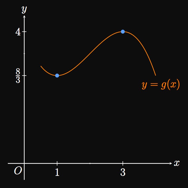
Locating the extrema—the minimum and maximum values—of a function is a vital skill in calculus. Let's begin with definitions. In Figure 1 we say \(g(1) = 8/3\) is the absolute minimum value of \(g\) because \((1, 8/3)\) is the lowest point on the graph. Conversely, \(g(3) = 4\) is the absolute maximum value of \(g\) because \((3, 4)\) is the highest point on the graph. Both \(g(1)\) and \(g(3)\) are called extrema of \(g.\) We formally define these terms as follows.
- absolute maximum (or global maximum) value of \(f\) if \(f(c) \geq f(x)\) for all \(x\) in \(D.\)
- absolute minimum (or global minimum) value of \(f\) if \(f(c) \leq f(x)\) for all \(x\) in \(D.\)
Many functions have both an absolute minimum and an absolute maximum, but some have just one or neither. The following examples demonstrate these cases.
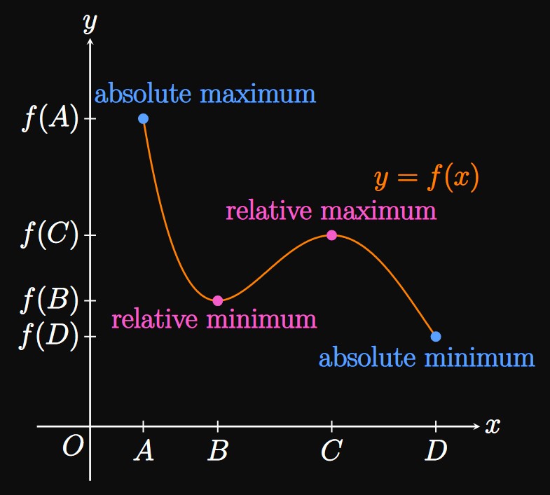
Relative Extrema The graphs of many functions have peaks and troughs. As an example, the graph of \(y = f(x)\) in Figure 4 has a peak at \((C, f(C))\) and a trough at \((B, f(B)).\) We call \(f(C)\) a relative maximum value of \(f\) because \(f(C)\) is the largest value for \(x\) near \(C.\) Similarly, \(f(B)\) is a relative minimum value of \(f\) since \(f(B)\) is the smallest value for \(x\) near \(B.\) But these numbers are not absolute extrema of \(f.\) Instead, \(f(A)\) is the absolute maximum value of \(f\) and \(f(D)\) is the absolute minimum value of \(f.\) Formally, we define relative extrema as follows.
- relative maximum value of \(f\) if \(f(c) \geq f(x)\) for \(x\) near \(c.\)
- relative minimum value of \(f\) if \(f(c) \leq f(x)\) for \(x\) near \(c.\)
The term local extremum
is interchangeable with relative extremum.
When we say \(x\) near \(c,\)
we mean it is true on an open interval containing \(c.\)
In Figure 4
\(f(B)\) is a relative minimum value of \(f\)
since it's the smallest value of \(f\) on some open interval containing \(B\)—say,
\((B - \delta, B + \delta)\) for sufficiently small \(\delta \gt 0.\)
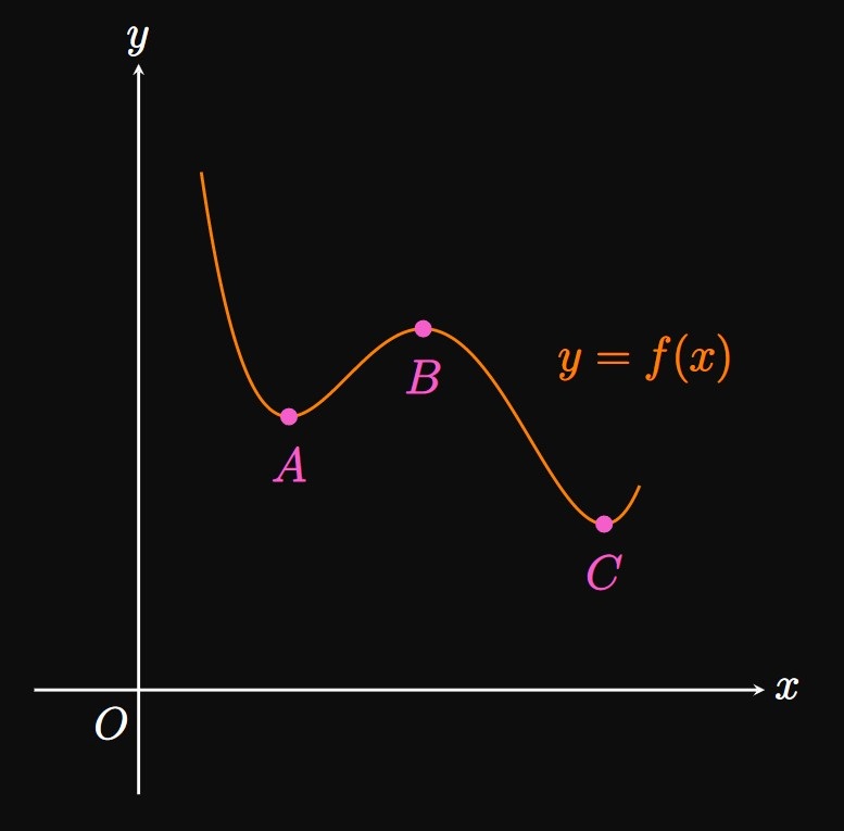
- a relative minimum at \(A.\)
- a relative maximum at \(B.\)
- a relative minimum and the absolute minimum at \(C.\)
Next we discuss a function's extrema on a closed interval. Instead of considering an entire graph, what if we just examine a portion? For example, in Example 2 we concluded that \(f(x) = x^3\) has no absolute extrema over its domain, \(\RR.\) But over the closed interval \([-1, 1],\) the absolute minimum of \(f(x) = x^3\) is \(f(-1) = -1\) and the absolute maximum is \(f(1) = 1.\) It therefore appears that any continuous function must have both an absolute minimum and an absolute maximum over a closed interval. This observation turns out to be true by the Extreme Value Theorem, defined below.
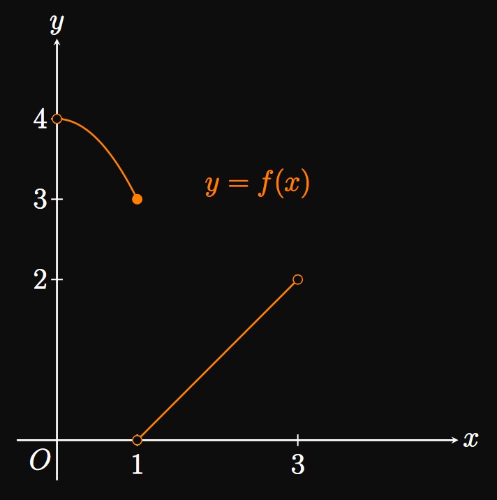
While intuitive, the Extreme Value Theorem turns out to be difficult to prove, so we omit the proof. Extreme values can be attained more than once, as shown by Example 4. We emphasize that both conditions of the Extreme Value Theorem—continuity and closed interval—must be satisfied. If either is omitted, then a function is not guaranteed to have any extrema. As an example, the graph of \(y = f(x)\) in Figure 7 is discontinuous and undefined at \(x = 0\) and \(x = 3.\) Thus, the Extreme Value Theorem bestows no guarantees that \(f\) has any extrema. Indeed, \(f\) has neither an absolute minimum nor an absolute maximum on \([0, 3].\)
Locating Extrema
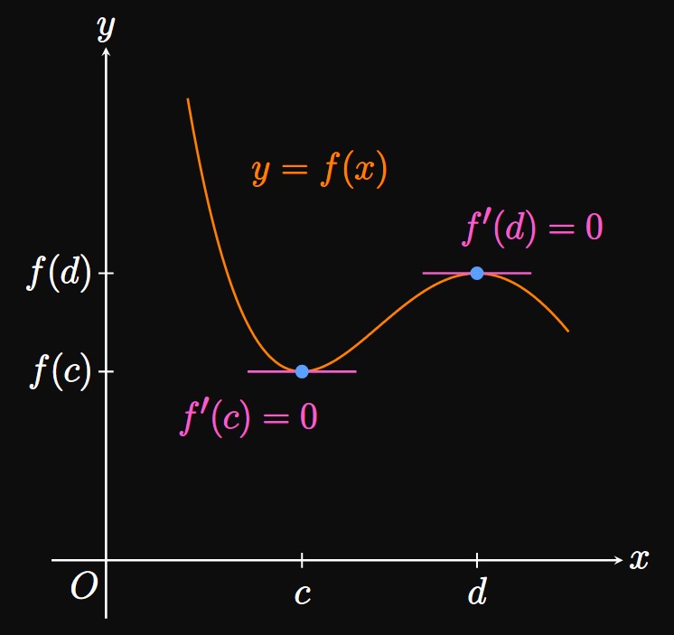
A connection exists between a function's extrema and its derivatives. As shown in Figure 8, the graph of \(y = f(x)\) has horizontal tangents at the relative minimum \((c, f(c))\) and at the relative maximum \((d, f(d)).\) Because the derivative is the slope of the tangent line, which is \(0,\) it follows that \(f'(c) = 0\) and \(f'(d) = 0.\) Simply put, the function's derivative equals \(0\) at a relative extremum. By Fermat's Theorem, defined below, this observation is always true for differentiable functions.
PROOF First suppose that \(f\) is differentiable at \(c.\) Then by the limit definition of a derivative (Section 2.1), \[ \ba f'(c) &= \lim_{h \to 0} \frac{f(c + h) - f(c)}{h} \nl &= \lim_{h \to 0^+} \frac{f(c + h) - f(c)}{h} \nl &= \lim_{h \to 0^-} \frac{f(c + h) - f(c)}{h} \pd \ea \] (A limit exists if and only if the one-sided limits exist and equal each other.) Next suppose that \(f\) has a relative maximum at \(c.\) Then \(f(c) \geq f(x)\) for \(x\) sufficiently close to \(c.\) Formally, if \(h\) is sufficiently close to \(0,\) with \(h\) either positive or negative, then \begin{flalign} &&f(c) &\geq f(c + h) \nonum &\nl \laWord{so} && f(c + h) - f(c) &\leq 0 \pd \label{eq:f-c-h-inequality} \end{flalign} For positive \(h,\) dividing both sides of \(\eqref{eq:f-c-h-inequality}\) by \(h\) yields \[ \frac{f(c + h) - f(c)}{h} \leq 0 \pd \] Taking the right-hand limit of both sides, we get \[ \lim_{h \to 0^+} \frac{f(c + h) - f(c)}{h} \leq \underbrace{\lim_{h \to 0^+} 0}_0 \pd \] But the limit on the left is simply \(f'(c),\) so we have \(f'(c) \leq 0.\) Conversely, if \(h \lt 0\) then we flip the inequality sign in \(\eqref{eq:f-c-h-inequality}\) after dividing by \(h \col\) \[\frac{f(c + h) - f(c)}{h} \geq 0 \pd\] Taking the left-hand limits of both sides produces \[ \lim_{h \to 0^-} \frac{f(c + h) - f(c)}{h} \geq \underbrace{\lim_{h \to 0^-} 0}_0 \pd \] Yet the left side is \(f'(c),\) so we attain \(f'(c) \geq 0.\) Accordingly, we have \(f'(c) \geq 0\) and \(f'(c) \leq 0;\) both can only be true if \(f'(c) = 0.\) Thus, Fermat's Theorem is proved for the case of a relative maximum at \(c.\) Proving Fermat's Theorem for the case of a relative minimum is performed similarly. \[\qedproof\]
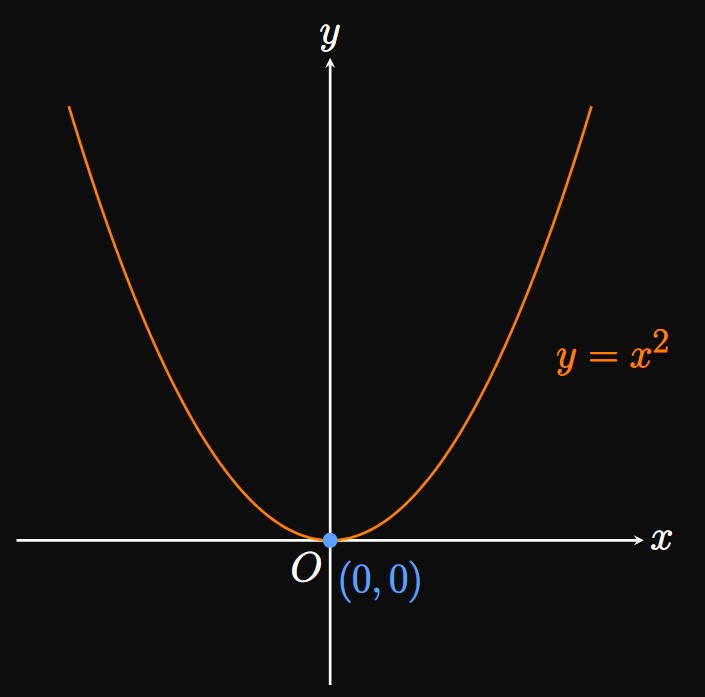
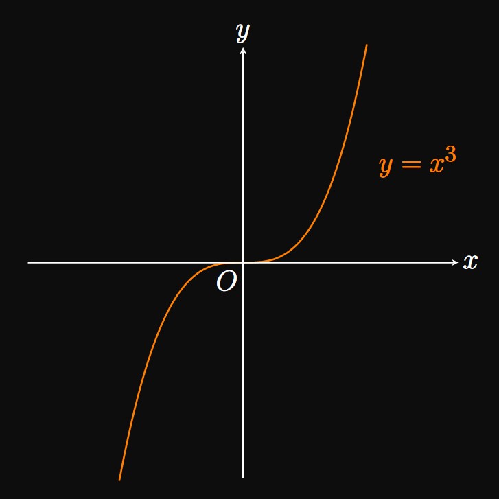
CAUTION The converse of Fermat's Theorem is not generally true: Just because \(f'(c) = 0\) does not mean \(f\) has a relative extremum at \(c.\) For example, if \(f(x) = x^3\) then \(f'(x) = 3x^2\) and \(f'(0) = 0.\) But \(x^3\) does not have an extremum at \(x = 0,\) as discussed in Example 2.

Instead, Fermat's Theorem says \(f\) could have a relative extremum at \(c\) if \(f'(c) = 0.\) Yet \(f\) may also have an extremum at \(c\) when \(f'(c)\) does not exist. For example, \(g(x) = \abs x\) has an absolute minimum (and a relative minimum) value at \(x = 0,\) even though \(g'(0)\) is undefined (Figure 9). Thus, to find the relative extrema of \(f,\) our objective is clear: We examine points at which \(f'(c) = 0\) or \(f'(c)\) does not exist. We call these \(c\) critical numbers, and the point \((c, f(c))\) is a critical point.
Thus, we can rephrase Fermat's Theorem as follows: if \(f\) has a relative extremum at \(c,\) then \(c\) is a critical number of \(f.\) Accordingly, finding a function's critical numbers allows us to locate its relative extrema.
CAUTION It is easy to forget that \(c\) must be within the domain of \(f.\) For example, the derivative of \(f(x) = 1/x\) is \(f'(x) = -1/x^2,\) which is undefined at \(x = 0.\) But since \(f(0)\) is also undefined, \(0\) is not a critical number of \(f.\)
We now present a coherent strategy for locating absolute extrema: If \(f\) is continuous over \([a, b],\) then \(f\) has both an absolute minimum value and an absolute maximum value in \([a, b]\) by the Extreme Value Theorem. The absolute extrema of \(f\) must either match the relative extrema or reside at the endpoints. Hence, the endpoints and critical numbers are possible locations of absolute extrema, so we must evaluate \(f\) at these values. This strategy is called the Closed Interval Method.
- Evaluate \(f\) at its critical numbers in \((a, b).\)
- Evaluate \(f\) at the endpoints \(a\) and \(b.\)
- Determine the smallest and largest of the values in Steps 1 and 2. The largest value is the absolute maximum of \(f,\) while the smallest value is the absolute minimum of \(f.\)
| \(x\) | \(-2\) | \(-1\) | \(2\) | \(4\) |
| \(g(x)\) | \(-2\) | \(7/2\) | \(-10\) | \(16\) |
Extrema Extrema (singular, extremum) are the minimum or maximum values of a function. A function \(f\) may have two types of extrema: absolute extrema (or global extrema) and relative extrema (or local extrema). If \(c\) is in the domain \(D\) of \(f,\) then \(f(c)\) is the
- absolute maximum (or global maximum) value of \(f\) if \(f(c) \geq f(x)\) for all \(x\) in \(D.\)
- absolute minimum (or global minimum) value of \(f\) if \(f(c) \leq f(x)\) for all \(x\) in \(D.\)
While many functions have both an absolute minimum and an absolute maximum, some have just one or no absolute extrema. Additionally, the value \(f(c)\) is a
- relative maximum value of \(f\) if \(f(c) \geq f(x)\) for \(x\) near \(c.\)
- relative minimum value of \(f\) if \(f(c) \leq f(x)\) for \(x\) near \(c.\)
Relative maxima correspond to peaks in the graph of \(f,\) while \(f\) has troughs at relative minima. By the Extreme Value Theorem, if \(f\) is continuous over \([a, b],\) then \(f\) attains an absolute minimum value \(f(c)\) and an absolute maximum value \(f(d),\) where \(c\) and \(d\) are in \([a, b].\)
Locating Extrema By Fermat's Theorem, if \(f\) has a relative extremum at \(c\) and \(f'(c)\) exists, then \(f'(c) = 0.\) Simply put, the graph of a differentiable function has horizontal tangents at its relative extrema. But the converse of Fermat's Theorem is not generally true: if \(f'(c) = 0,\) then \(f\) doesn't need to have a relative extremum at \(c.\) Critical numbers \(c\) in the domain of \(f\) satisfy \(f'(c) = 0\) or \(f'(c)\) failing to exist. Then \((c, f(c))\) is called a critical point. The Closed Interval Method provides the following guide for locating absolute extrema on an interval \([a, b].\)
- Evaluate \(f\) at the critical numbers in \((a, b).\)
- Evaluate \(f\) at the endpoints \(a\) and \(b.\)
- Determine the smallest and largest of the values in Steps 1 and 2. The largest value is the absolute maximum of \(f,\) while the smallest value is the absolute minimum of \(f.\)