2.8: Linearization and Differentials
When we first introduced derivatives in Section 2.1, we declined to elaborate on differentials. In Section 2.2, we wrote equations of tangent lines. In this section we use tangent lines to approximate a function's outputs. We also define differentials and provide applications for them, including how they are connected to tangent lines. This section covers the following topics:
Linearization
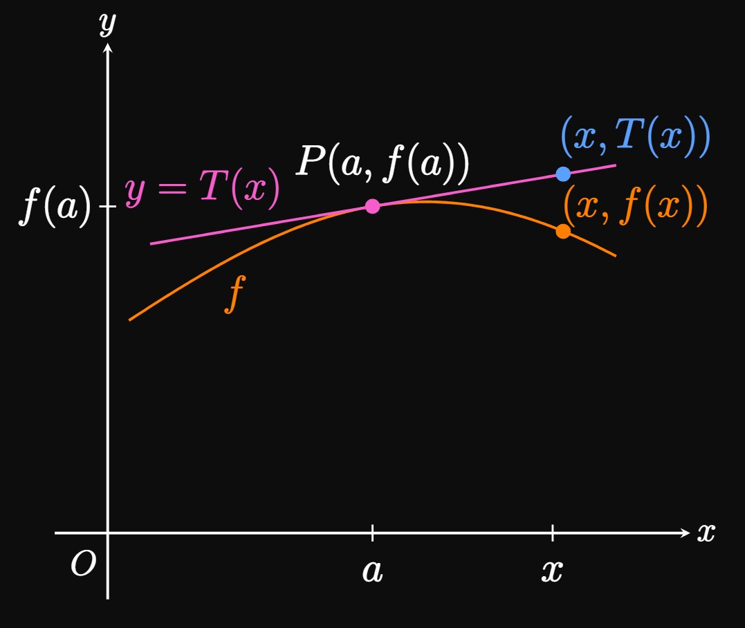
When we have a complicated function, it could be difficult to compute its outputs explicitly. But we can use calculus to approximate its values by using a line. The best linear approximation of a function is its tangent line. This process is called linearization—the procedure of estimating a function's values by using the outputs of its tangent line. In other words, we approximate a curve to be its tangent line. Suppose that a line is tangent to the curve \(f\) at the point \(P(a, f(a)).\) Let \(T(x)\) be the function that represents this tangent line. In Section 2.2 we asserted that an equation of this tangent line is \[y - f(a) = f'(a) (x - a) \pd\] Replacing \(y\) with \(T(x)\) gives \[T(x) = f(a) + f'(a)(x - a) \pd\] We take \(T(x)\) to estimate \(f(x),\) so we use \begin{equation} f(x) \approx f(a) + f'(a) (x - a) \pd \label{eq:f-approx} \end{equation} Figure 1 shows the line tangent to the curve \(f\) at the point \(P(a, f(a)).\) The point \((x, T(x))\) on the line approximates \((x, f(x)).\) We say the linearization of \(f(x)\) is centered at \(x = a\) because we use this point as a reference for the approximation; note that \(T(a) = f(a).\) In this estimate, we are assuming that \(f\) changes consistently at the same rate \(f'(a).\) This approximation for \(f\) is effective for \(x\) near the point of tangency, \(P,\) because zooming in on the curve \(f\) near \(P\) reveals a resemblance to a line. But this approximation often diminishes in accuracy for \(x\) far away from \(P.\)
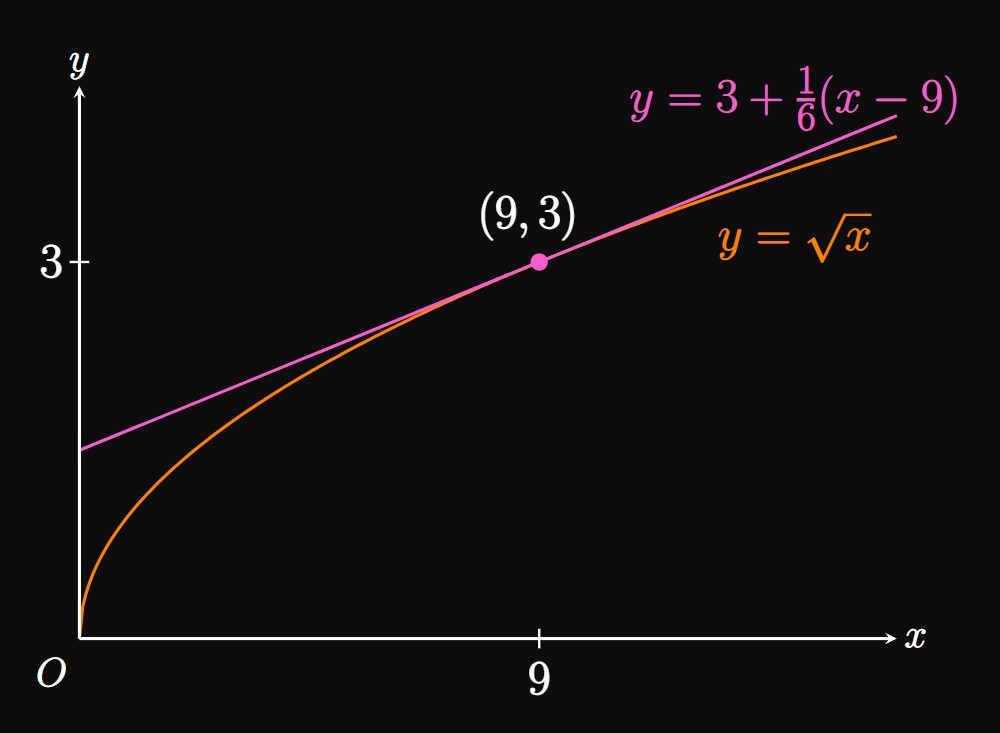
Equation of Tangent Line To calculate the slope of \(y = \sqrt x\) when \(x = 9,\) we differentiate \(\sqrt x = x^{1/2}\) using the Power Rule: \[\deriv{}{x} \par{x^{1/2}} = \tfrac{1}{2} x^{-1/2} = \frac{1}{2 \sqrt x} \pd\] Hence, the slope when \(x = 9\) is \[\frac{1}{2 \sqrt 9} = \frac{1}{6} \pd\] The point of tangency is \((9, 3),\) so an equation of the tangent line is \[y - 3 = \tfrac{1}{6} (x - 9) \or \boxed{y = 3 + \tfrac{1}{6} (x - 9)}\] (See Figure 2.)
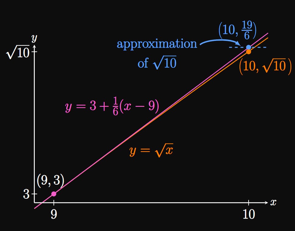
Approximation The tangent line \(y = 3 + \tfrac{1}{6} (x - 9)\) is the best linear approximation to \(y = \sqrt x\) for \(x\) near \(9.\) We estimate \(\sqrt{10}\) as the output of this tangent line when \(x = 10.\) Substituting \(x = 10\) into the equation of the tangent line, we see \[\sqrt{10} \approx 3 + \tfrac{1}{6}(10 - 9) = \boxed{\tfrac{19}{6}} \approx 3.167 \pd\] The actual value of \(\sqrt{10}\) is approximately \(3.162.\) Our approximation of \(3.167\) is very accurate! Since \(x = 10\) is close to the center of the approximation, \(a = 9,\) the tangent line is an excellent estimate for the value of \(\sqrt x.\) (See Figure 3.) Using tangent lines allows you to estimate values of square roots in your head—a great trick.
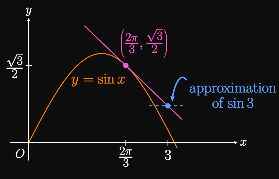
Equation of Tangent Line The derivative of \(\sin x\) is \(\cos x,\) so the slope of the curve \(y = \sin x\) at \(x = 2 \pi/3\) is \[\cos \frac{2 \pi}{3} = -\frac{1}{2} \pd\] When \(x = 2 \pi/3,\) \[y = \sin \frac{2 \pi}{3} = \frac{\sqrt 3}{2} \pd\] Thus, an equation of the tangent line is \[y - \frac{\sqrt 3}{2} = -\frac{1}{2} \par{x - \frac{2 \pi}{3}} \or \boxed{y = -\frac{x}{2} + \frac{\pi}{3} + \frac{\sqrt 3}{2}} \]
Approximation We approximate \(\sin 3\) as the \(y\)-value the tangent line reaches when \(x = 3.\) Substituting \(x = 3\) into the equation of the tangent line shows that \[\sin 3 \approx -\frac{1}{2} (3) + \frac{\pi}{3} + \frac{\sqrt 3}{2} \approx \boxed{0.413}\] Unfortunately, the actual value of \(\sin 3\) turns out to be roughly \(0.141.\) Our estimate \(0.413\) is not very accurate because \(x = 3\) is relatively far away from the center of the linearization, \(x = 2 \pi/3.\) (See Figure 4.)
Differentials
Until now, we have postponed the interpretation of the differentials \(\dd x\) and \(\dd y\) in the equation \(\textDeriv{y}{x} = f'(x).\) Multiplying both sides by \(\dd x\) shows \begin{equation} \dd y = f'(x) \di x \pd \label{eq:dy-dx} \end{equation} In this form, we interpret \(\dd x\) as an independent variable whose value we are free to select. Then \(\dd y\) is a corresponding dependent variable whose value depends on \(x\) and \(\dd x.\) Notice that small values of \(\dd x\) yield small outputs \(\dd y,\) whereas large values of \(\dd x\) force \(\dd y\) to be more substantial.
- \(\dd \par{\sin x}\)
- \(\dd \par{y^4}\)
- \(\dd \par{t e^t}\)
- The derivative of \(\sin x\) is \(\cos x,\) so we say \[\dd \par{\sin x} = \boxed{\cos x \di x}\]
- By the Power Rule, the derivative of \(y^4\) is \(4y^3.\) So \[\dd \par{y^4} = \boxed{4y^3 \di y}\]
- The Product Rule gives the derivative of \(te^t\) to be \(e^t + te^t.\) Thus, \[\dd \par{t e^t} = \boxed{\par{e^t + te^t} \di t}\]
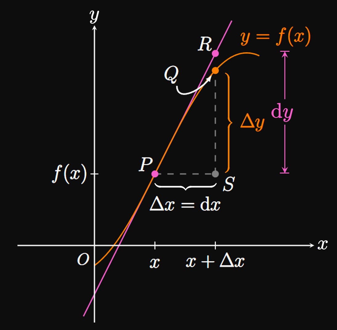
Interpreting Differentials Geometrically Differentials model the slope of a tangent line. In Figure 5, the points \(P(x, f(x))\) and \(Q(x + \Delta x, f(x + \Delta x))\) are marked on the graph of \(f.\) The line tangent to \(f\) at \(P\) is drawn. Segment \(\segment{PS}\) is the change in \(x\) over the interval \([x, x + \Delta x];\) we take \(\Delta x = \dd x.\) Observe that the change in the \(y\)-value of \(f\) over \([x, x + \Delta x]\) is given by \[\Delta y = f(x + \Delta x) - f(x) = \length{QS} \pd\] Over the interval \([x, x + \Delta x],\) the tangent line rises by a height \(\segment{RS}.\) Since this tangent line has slope \(f'(x),\) its rise \(\length{RS}\) is given by \begin{equation} \dd y = f'(x) \di x \pd \eqlabel{eq:dy-dx} \end{equation} Thus, \(\dd y\) is the amount by which the tangent line rises or falls, whereas \(\Delta y\) measures the amount by which the curve \(f\) rises or falls. As an example, in Figure 1 over the interval \([a, x],\) the curve \(f\) falls but the tangent line rises; hence, \(\Delta y \lt 0\) but \(\dd y \gt 0.\) As \(\dd x\) is made smaller, the approximation \(\Delta y \approx \dd y\) increases in accuracy; that is, the amount by which the tangent line rises or falls follows the amount risen or fallen by the curve. Therefore, we often think of \(\dd x\) and \(\dd y\) as infinitely small quantities—such that the curve behaves approximately to its tangent line. Doing so enables us to approximate values of \(f\) (whose identity could be difficult to obtain) as the values of its tangent line.
If we desire, then we can use \(\eqref{eq:dy-dx}\) as a linear approximation. In fact, \(\eqref{eq:dy-dx}\) is an alternate representation of \(\eqref{eq:f-approx},\) as shown by the following algebra: Taking \(\dd y \approx \Delta y\) and \(\dd x = \Delta x\) at \(a,\) \(\eqref{eq:dy-dx}\) becomes \begin{flalign} &&\Delta y &\approx f'(a) \Delta x \nonumber &\nl \laWord{or} && f(x) - f(a) &\approx f'(a)(x - a) \nonumber &\nl \laWord{so} && f(x) &\approx f(a) + f'(a) (x - a) \pd \eqlabel{eq:f-approx} \end{flalign} Thus, differentials present another (yet equivalent) perspective to linear approximations.
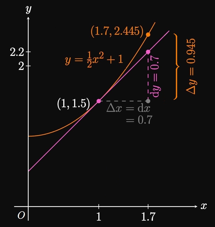
From \(1\) to \(1.7\) We see \[\deriv{}{x} \par{\tfrac{1}{2} x^2 + 1} = x \pd\] Therefore, the differential \(\dd y\) is given by \begin{equation} \dd y = x \di x \pd \label{eq:dy-ex} \end{equation} Because \(x\) changes from \(1\) to \(1.7,\) we take \(\dd x = 0.7\) and so \(\eqrefer{eq:dy-ex}\) gives \[\dd y = (1)(0.7) = \boxed{0.7}\] Conversely, we see \[ \ba \Delta y &= \parbr{\tfrac{1}{2} (1.7)^2 + 1} - \parbr{\tfrac{1}{2} (1)^2 + 1} \nl &= \boxed{0.945} \ea \] (See Figure 6.)
From \(1\) to \(1.2\) Since \(x\) changes from \(1\) to \(1.2,\) we use \(\dd x = 0.2.\) By \(\eqref{eq:dy-ex},\) \[\dd y = (1)(0.2) = \boxed{0.2}\] In contrast, \[ \ba \Delta y &= \parbr{\tfrac{1}{2} (1.2)^2 + 1} - \parbr{\tfrac{1}{2} (1)^2 + 1} \nl &= \boxed{0.22} \ea \] Note that \(\dd y\) is much easier to compute than \(\Delta y.\) We see that \(\Delta y \approx \dd y\) increases in accuracy for small values of \(\dd x.\) For example, the difference between \(\dd y\) and \(\Delta y\) is even smaller if \(x\) changes from \(1\) to \(1.1.\) For small values of \(\dd x,\) the tangent line to \(y = \tfrac{1}{2} x^2 + 1\) at \(x = 1\) becomes nearly indistinguishable from the curve.
Maximum Error Let \(r\) be the sphere's radius and \(V\) be its volume. Then \(V = \tfrac{4}{3} \pi r^3.\) We take the maximum measurement error of \(r\) to be \(\Delta r = \dd r.\) Likewise, the error in \(V\) is \(\Delta V,\) as approximated by \[\dd V = 4 \pi r^2 \di r \pd\] For \(r = 14\) and \(\dd r = 0.07,\) we estimate the maximum error in the sphere's volume to be \[\dd V = 4 \pi(14)^2 (0.07) \approx \boxed{172.411 \un{cm}^3}\]
Percent Error The relative error is given by the error \(\Delta V\) divided by the measured volume \(V.\) The sphere's volume is measured to be \[V = \tfrac{4}{3} \pi r^3 = \tfrac{4}{3} \pi (14)^3 \approx 11494.040 \un{cm}^3 \pd\] Hence, the maximum relative error in the measurement is \[ \frac{\Delta V}{V} \approx \frac{\dd V}{V} = \frac{172.411}{11494.040} \approx 0.015 \pd \] This relative error is equivalent to a percent error of \(\boxed{1.500\%}.\)
Linearization We use linearization to approximate a function's values by constructing a tangent line. If \(f\) is differentiable at \(a,\) then we form a tangent line to \(f\) at \(a\) (the center of the approximation). Then we approximate \(f(x)\) by evaluating its tangent line at \(x \col\) \begin{equation} f(x) \approx f(a) + f'(a) (x - a) \pd \eqlabel{eq:f-approx} \end{equation} Linearization is the best linear approximation of \(f(x),\) and it is effective for \(x\) close to \(a.\)
Differentials If \(y = f(x)\) and \(f\) is differentiable, then the differential \(\dd y\) is given by \begin{equation} \dd y = f'(x) \di x \pd \eqlabel{eq:dy-dx} \end{equation} Geometrically, \(\dd y\) is the amount by which the tangent line to \(f\) at \(x\) rises or falls as \(x\) is increased by \(\dd x.\) Differentials present another way to perform linear approximations and are useful for estimating the maximum errors of measurements.