2.2: Differentiating Power, Exponential, and Sinusoidal Functions
In Section 2.1 we formed a relationship between derivative functions and slopes to a graph. We now find derivative functions of several important functions—power functions, exponential functions, and sinusoidal functions. We discuss the following topics:
- Power Rule
- Equations of Tangent Lines and Normal Lines
- Differentiating \(e^x\)
- Derivatives of Sine and Cosine
Power Rule
Let's investigate the family of functions \(f(x) = x^n\) where \(n\) is any real number. This family is called a power function. In Section 2.1 we discovered that \[\deriv{}{x} \par{x^2} = 2x \and \deriv{}{x} \par{x^3} = 3x^2 \pd\] Using the limit definition of a derivative also shows that the derivative of \(x^4\) is \(4x^3.\) We see a pattern emerging—the derivative function is found by multiplying the function by the power and then subtracting \(1\) from the exponent. Thus, the following rule seems apparent: Differentiating \(f(x) = x^n\) is very easy if we use the Power Rule, which states \begin{equation} \deriv{}{x} \par{x^n} = nx^{n - 1} \pd \label{eq:power-rule} \end{equation} The Power Rule turns out to be true for all real \(n,\) not just integers, and is proved in Appendix A.2.
- \(\ds \deriv{}{x} \par{x^6}\)
- \(\ds \deriv{}{x} \par{\frac{1}{x^4}}\)
- \(\ds \deriv{}{x} \par{\sqrt[4]{x^3} \,}\)
- We use the Power Rule, as in \(\eqref{eq:power-rule},\) with \(n = 6.\) We drop the power and then subtract \(1\) from the exponent, so the derivative becomes \[6x^{6 - 1} = \boxed{6x^5}\]
- We rewrite the function as \(x^{-4},\) so we use \(\eqref{eq:power-rule}\) with \(n = -4\) to obtain \[-4x^{-4 - 1} = -4x^{-5} = \boxed{-\frac{4}{x^5}}\]
- Upon rewriting the function as \(x^{3/4},\) we identify \(n = 3/4\) and so \(\eqref{eq:power-rule}\) gives the derivative to be \[\tfrac{3}{4} x^{-1/4} = \boxed{\frac{3}{4 \sqrt[4]{x}}}\]
Sums and Differences of Power Functions We use the Sum Rule and Difference Rule for Derivatives (from Section 2.1) to differentiate sums and differences of power functions. For example, a polynomial is the sum (or difference) of power functions whose exponents are nonnegative integers. Thus, to differentiate a polynomial we use the Sum and Difference Rules in conjunction with the Power Rule. Doing so provides a faster method of differentiation than using the limit definition of a derivative.
- \(\ds \deriv{}{x} \par{x^2 - x}\)
- \(\ds \deriv{}{x} \par{\frac{3}{x} + 2}\)
- \(\ds \deriv{}{x} \par{4x \sqrt x \,}\)
- By the Difference Rule for Derivatives, \[\deriv{}{x} \par{x^2 - x} = \deriv{}{x} \par{x^2} - \deriv{}{x} \par{x} \pd\] Using the Power Rule for each term on the right-hand side, we see \[ \deriv{}{x} \par{x^2} = 2x \and \deriv{}{x} \par{x} = 1 \pd \] Hence, \[\deriv{}{x} \par{x^2 - x} = \boxed{2x - 1}\]
- This derivative requires several differentiation rules: \[ \ba \deriv{}{x} \par{\frac{3}{x} + 2} &= \deriv{}{x} \par{\frac{3}{x}} + \deriv{}{x} \par{2} &&(\textrm{Sum Rule}) \nl &= \deriv{}{x} \par{\frac{3}{x}} + 0 &&(\textrm{Constant Rule}) \nl &= \deriv{}{x} \par{3x^{-1}} \nl &= 3 \deriv{}{x} \par{x^{-1}} &&(\textrm{Constant Multiple Rule}) \nl &= 3 \par{-1 x^{-2}} &&(\textrm{Power Rule}) \nl &= \boxed{-\frac{3}{x^2}} \ea \]
- We rewrite \(\sqrt x\) as \(x^{1/2},\) so \(x \sqrt x\) becomes \[x \cdot x^{1/2} = x^{3/2} \cma\] which is a power function. Thus, we have \[ \ba \deriv{}{x} \par{4x \sqrt x \,} &= \deriv{}{x} \par{4x^{3/2}} \nl &= 4 \deriv{}{x} \par{x^{3/2}} && (\textrm{Constant Multiple Rule}) \nl &= 4 \par{\tfrac{3}{2} x^{1/2}} && (\textrm{Power Rule}) \nl &= 6x^{1/2} = \boxed{6 \sqrt x} \ea \]
Equations of Tangent Lines and Normal Lines
Tangent Lines Suppose that the function \(f\) is differentiable at the point \(P(a, f(a)).\) We know that \(f'(a)\) measures the slope of the line tangent to \(f\) at \(P.\) To provide an equation of this tangent line, we use the point-slope form for the equation for a line: If a line passes through a point \(\par{x_0, y_0}\) with slope \(m,\) then its equation is given by \[y - y_0 = m \par{x - x_0} \pd\] Since the tangent line to \(f\) passes through \(\par{x_0, y_0}\) \(=(a, f(a))\) with slope \(m = f'(a),\) an equation of the tangent line to \(f\) at \(x = a\) is given by \begin{equation} y - f(a) = f'(a) \par{x - a} \pd \label{eq:tan-line} \end{equation}
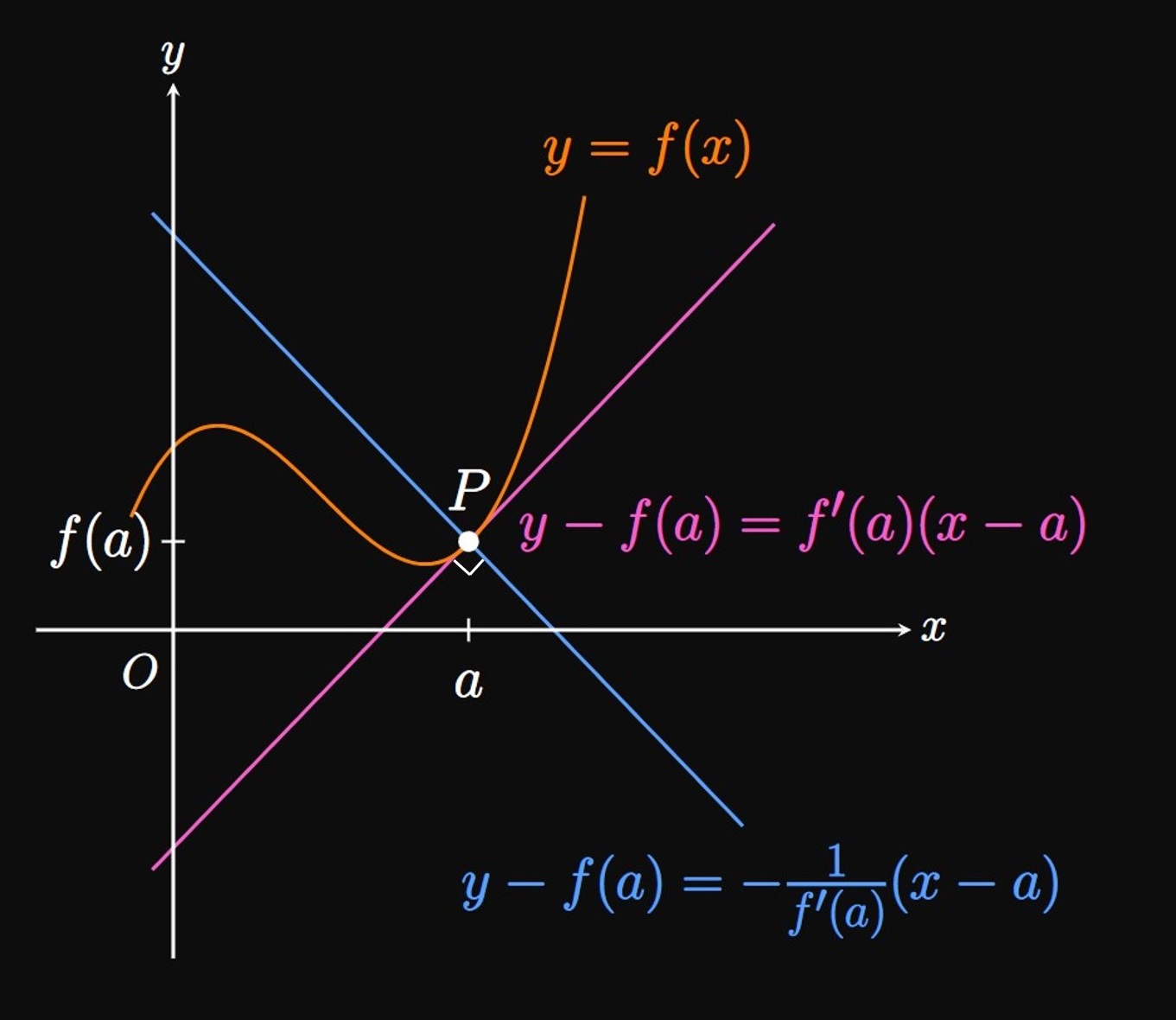
Normal Lines A line is called normal to a curve \(y = f(x)\) at point \(P(a, f(a))\) if the line intersects \(P\) at an angle of \(90\degree\) to the curve. Therefore, a normal line is perpendicular to a tangent line. If two lines are perpendicular to each other, then one of their slopes is the negative reciprocal of the other. Thus, the normal line to \(f\) at \(x = a\) has slope \(-1/f'(a)\) if \(f'(a) \ne 0.\) We preserve the same point \((a, f(a)),\) so in \(\eqref{eq:tan-line}\) we replace \(f'(a)\) with \(-1/f'(a).\) Doing so gives an equation for the line normal to \(f\) at \(P\) to be \begin{equation} y - f(a) = -\frac{1}{f'(a)}(x - a) \pd \label{eq:normal-line} \end{equation} (See Figure 2.)
We need the slope of the tangent line to the curve when \(x = 1.\) Thus, we differentiate the given function by using a combination of differentiation rules, as follows: \[ \ba \deriv{}{x} \par{x^2 - 4x + 4} &= \deriv{}{x} \par{x^2} - \deriv{}{x} \par{4x} + \deriv{}{x} \par{4} &&(\textrm{Sum and Difference Rules}) \nl &= \deriv{}{x} \par{x^2} - \deriv{}{x} \par{4x} + 0 &&(\textrm{Constant Rule}) \nl &= \deriv{}{x} \par{x^2} - 4 \deriv{}{x} \par{x} &&(\textrm{Constant Multiple Rule}) \nl &= 2x - 4 \pd &&(\textrm{Power Rule}) \ea \] When \(x = 1,\) the slope of the line tangent to the curve is \[2(1) - 4 = -2 \pd\] Also note that when \(x = 1,\) \[y = (1)^2 - 4(1) + 4 = 1 \pd\] Hence, the point of tangency is \((1, 1).\)
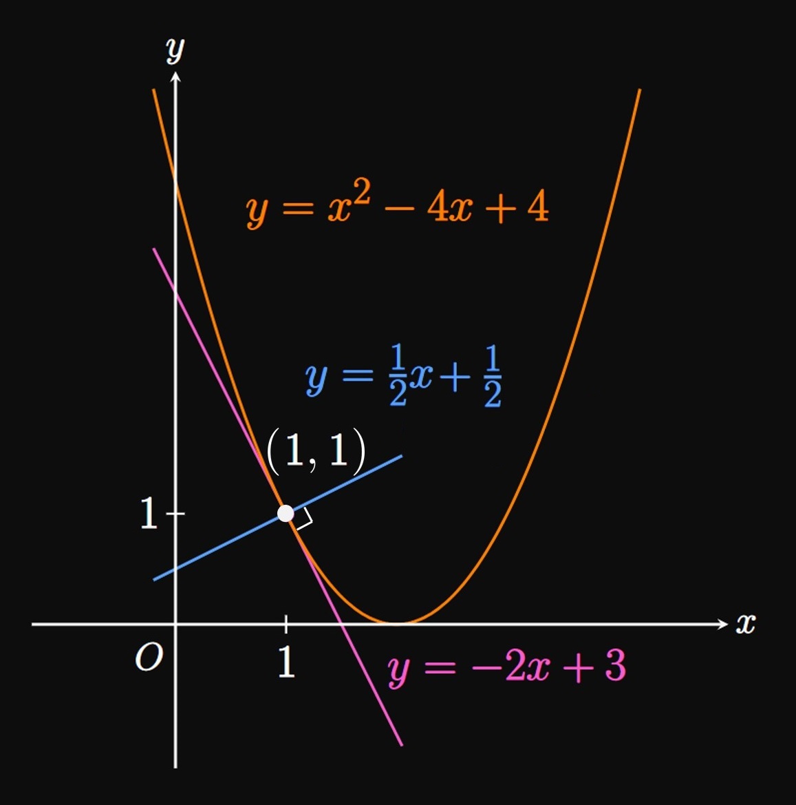
Equation of Tangent Line The tangent line just touches the curve at the point of tangency \((1, 1)\) with slope \(-2.\) Thus, we use the point-slope form for the equation of a line: \(\eqrefer{eq:tan-line}\) gives the equation of the tangent line to be \[ y - 1 = -2(x - 1) \or \boxed{y = -2x + 3} \]
Equation of Normal Line The normal line strikes the point \((1, 1)\) at an angle of \(90 \degree\) with the curve. Thus, the normal line is perpendicular to the tangent line. Since the tangent line has slope \(-2,\) the normal line has slope \(1/2\) (the negative reciprocal). The point-slope form for the equation of a line, as in \(\eqref{eq:normal-line},\) represents this normal line as \[ y - 1 = \tfrac{1}{2} (x - 1) \or \boxed{y = \tfrac{1}{2} x + \tfrac{1}{2}} \] (See Figure 3.)
Differentiating \(e^x\)

Whereas in power functions the base is a variable, in exponential functions the power is a variable. Recall that the domain of an exponential function is all real numbers; an example of an exponential function is \(b^x\) for any \(b \gt 0.\) The Power Rule cannot be used to differentiate an exponential function, since the rule is only applicable when the power is constant. We now discuss the derivative of an exponential function whose base is Euler's number, \[e \approx 2.718281828459045235936 \cma\] which satisfies a myriad of beautiful properties in mathematics. This number manages to present itself in many surprising applications in ecology, physics, and finance. One of these majestic properties is that the function \(e^x\) has its own derivative. In other words, the slope of the curve \(e^x\) equals itself—that is, \begin{equation} \deriv{}{x} \par{e^x} = e^x \pd \label{eq:deriv-e^x} \end{equation} In Figure 4, point \(P\) represents the point \((a, e^a)\) for any \(a.\) At \(P\) the slope of the tangent line is \(e^a,\) meaning that the curve's height is equal to its slope. In later sections, we will apply the premise of \(\eqref{eq:deriv-e^x}\) to differentiate functions whose bases aren't \(e,\) as we will see in Section 2.4.
PROOF Using the limit definition of a derivative, \[ \ba \deriv{}{x} \par{e^x} &= \lim_{h \to 0} \frac{e^{x + h} - e^x}{h} \nl &= \lim_{h \to 0} \frac{e^x \, e^h - e^x}{h} \nl &= \lim_{h \to 0} e^x \frac{e^h - 1}{h} \pd \ea \] Because \(e^x\) doesn't depend on \(h,\) the Constant Multiple Law for Limits (from Section 1.2) enables us to pull out the term \(e^x;\) we attain \begin{equation} \deriv{}{x} \par{e^x} = e^x \lim_{h \to 0} \frac{e^h - 1}{h} \pd \label{eq:deriv-lim} \end{equation} But what is the value of the limit on the right-hand side? The limit must be \(1\) so that \(\eqref{eq:deriv-e^x}\) holds true; in fact, \(e\) is the number for which \begin{equation} \lim_{h \to 0} \frac{e^h - 1}{h} = 1 \pd \label{eq:e-lim} \end{equation} Then \(\eqref{eq:deriv-lim}\) becomes \[\deriv{}{x} \par{e^x} = e^x \cdot 1 = e^x \pd\] Any other number wouldn't produce such a clean derivative function, as we will see in Section 2.4. For this reason, we work with \(e\) in calculus. \[\qedproof\]
The equations of the tangent line and normal line all require the slope of \(e^x\) when \(x = 2.\) We find this slope to be \[\deriv{}{x} \par{e^x} \intEval_{x = 2} = e^2 \pd\]
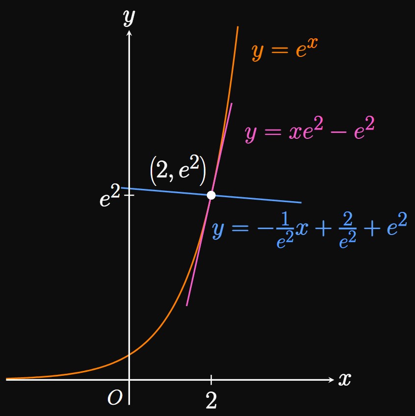
Equation of Tangent Line The tangent line intersects the curve at the point \(\par{2, e^2}.\) Accordingly, \(\eqref{eq:tan-line}\) gives an equation for the tangent line to be \[y - e^2 = e^2(x - 2) \or \boxed{y = xe^2 - e^2}\]
Equation of Normal Line The normal line strikes through the curve at \(\par{2, e^2}\) and is perpendicular to the tangent line. Hence, the slope of the normal line is the negative reciprocal of the slope of the tangent line—namely, \(-1/e^2.\) So using \(\eqref{eq:normal-line},\) we find an equation of the normal line to be \[y - e^2 = -\frac{1}{e^2} (x - 2) \or \boxed{y = -\frac{1}{e^2} x + \frac{2}{e^2} + e^2}\] (See Figure 5.)
Derivatives of Sine and Cosine
The functions \(y = \sin x\) and \(y = \cos x\) are called sinusoidal functions, which are continuous for all real numbers \(x.\) (Let's be clear that \(x\) is expressed in radians.) Each function's graph resembles repeating waves; thus, if we plot the values of the slopes of a curve at each \(x,\) then we expect the resulting curve to also resemble waves. Hence, we assume that the derivative of a sinusoidal function is another sinusoidal function. This expectation happens to be true: The derivative of sine is cosine, and the derivative of cosine is negative sine—that is, \begin{flalign} &&\deriv{}{x} \par{\sin x} &= \cos x \label{eq:deriv-sin} &\nl \laWord{and} &&\deriv{}{x} \par{\cos x} &= - \sin x \label{eq:deriv-cos} \pd \end{flalign} These formulas further strengthen the bond between sine and cosine.
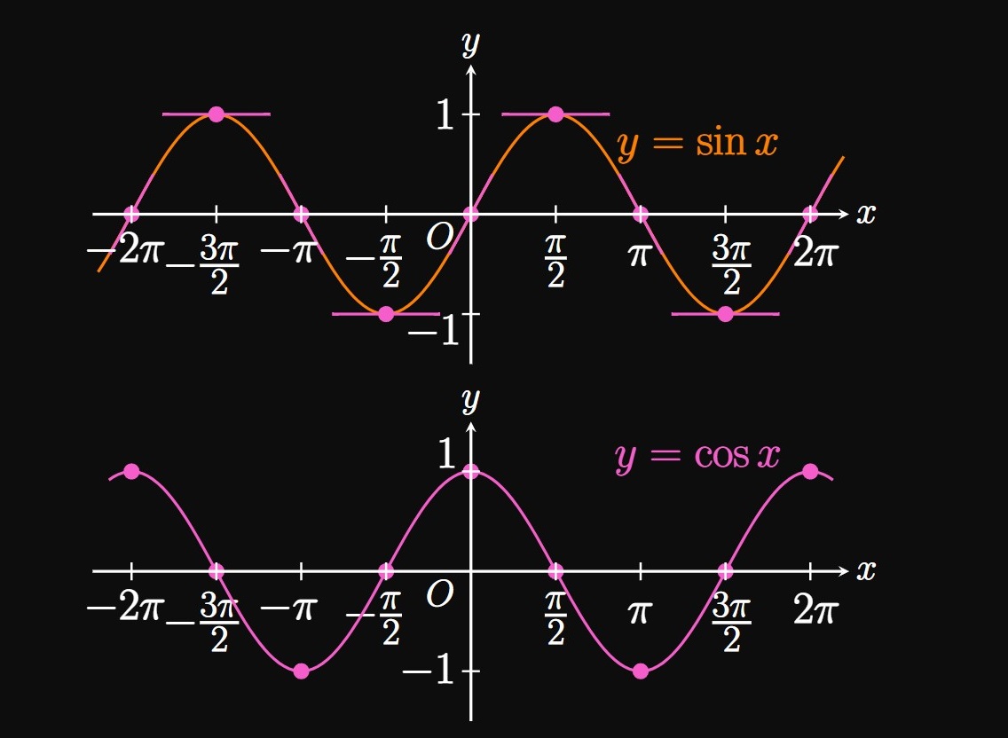
\(\eqrefer{eq:deriv-sin}\) asserts that the slope of \(y = \sin x\) at any \(x = a\) is \(\cos a.\) We now interpret this relationship geometrically: In the interval \([-2 \pi, 2\pi],\) the graph of \(\sin x\) has horizontal tangents when \(x = -3 \pi/2,\) \(x = -\pi/2,\) \(x = \pi/2,\) and \(x = 3 \pi/2.\) Thus, at these values the derivative of \(\sin x\) must be \(0;\) indeed, \(\cos x = 0\) at these values. Since \(\cos 0 = 1,\) the graph of \(\sin x\) has slope \(1\) when \(x = 0.\) The sine graph has positive slope over the interval \(\par{-\pi/2, \pi/2};\) indeed, \(\cos x \gt 0\) in this interval. (See Figure 6.) These observations enable us to guess that \(\eqref{eq:deriv-sin}\) is true.
PROOF OF \(\eqref{eq:deriv-sin}\) The derivative of \(\sin x,\) according to the limit definition of a derivative, is given by \[\deriv{}{x} \par{\sin x} = \lim_{h \to 0} \frac{\sin(x + h) - \sin x}{h} \pd\] To evaluate this limit, we expand the term \(\sin(x + h)\) using the addition identity for sine: \[ \ba \deriv{}{x} \par{\sin x} &= \lim_{h \to 0} \frac{\sin x \cos h + \cos x \sin h - \sin x}{h} \nl &= \lim_{h \to 0} \frac{(\sin x) (\cos h - 1) + \cos x \sin h}{h} \pd \ea \] The Sum Law for Limits (from Section 1.2) enables us to write \[ \deriv{}{x} \par{\sin x} = \lim_{h \to 0} \frac{\sin x(\cos h - 1)}{h} + \lim_{h \to 0} \frac{\cos x \sin h}{h} \pd \] Notice that \(\sin x\) and \(\cos x\) don't depend on \(h,\) so the Constant Multiple Law for Limits permits us to factor them outside of the limit expressions. We therefore attain \begin{equation} \deriv{}{x} \par{\sin x} = (\sin x) \lim_{h \to 0} \frac{\cos h - 1}{h} + (\cos x) \lim_{h \to 0} \frac{\sin h}{h} \pd \label{eq:sin-deriv-lim} \end{equation} In Section 1.2 we proved that \begin{equation} \lim_{h \to 0} \frac{\sin h}{h} = 1 \and \lim_{h \to 0} \frac{1 - \cos h}{h} = 0 \pd \label{eq:important-limits} \end{equation} It now becomes apparent why we studied these limits—\(\eqref{eq:sin-deriv-lim}\) becomes \[ \ba \deriv{}{x} \par{\sin x} &= (\sin x) \cdot 0 + (\cos x) \cdot 1 \nl &= \cos x \pd \ea \] \[\qedproof\]
PROOF OF \(\eqref{eq:deriv-cos}\) By the limit definition of a derivative, the derivative of cosine is represented by \[\deriv{}{x} \par{\cos x} = \lim_{h \to 0} \frac{\cos(x + h) - \cos x}{h} \pd\] To evaluate this limit, we expand the term \(\cos(x + h)\) using the addition identity for cosine: \[ \ba \deriv{}{x} \par{\cos x} &= \lim_{h \to 0} \frac{\cos x \cos h - \sin x \sin h - \cos x}{h} \nl &= \lim_{h \to 0} \frac{(\cos x) (\cos h - 1) - \sin x \sin h}{h} \pd \ea \] By the Difference Law for Limits (from Section 1.2), we observe \[\deriv{}{x} \par{\cos x} = \lim_{h \to 0} \frac{(\cos x) (\cos h - 1)}{h} - \lim_{h \to 0} \frac{\sin x \sin h}{h} \pd\] The factors \(\cos x\) and \(\sin x\) can be factored out of each limit by the Constant Multiple Law for Limits; doing so shows \[\deriv{}{x} \par{\cos x} = (\cos x) \lim_{h \to 0} \frac{\cos h - 1}{h} - (\sin x) \lim_{h \to 0} \frac{\sin h}{h} \pd\] Applying the formulas of \(\eqref{eq:important-limits}\) yields \[ \ba \deriv{}{x} \par{\cos x} &= (\cos x) \cdot 0 - (\sin x) \cdot 1 \nl &= - \sin x \pd \ea \] \[\qedproof\]
These proofs are elegant because they connect several key concepts: In Section 1.2 we introduced the Squeeze Theorem and used it to prove the limits in \(\eqref{eq:important-limits}.\) They immediately proved useful as we calculated indeterminate limits involving trigonometric functions. But in this section, we discovered more hidden applications of these limits. Through formulas \(\eqref{eq:deriv-sin}\) and \(\eqref{eq:deriv-cos},\) we appreciate how differential calculus further links the twin functions \(\sin x\) and \(\cos x.\)
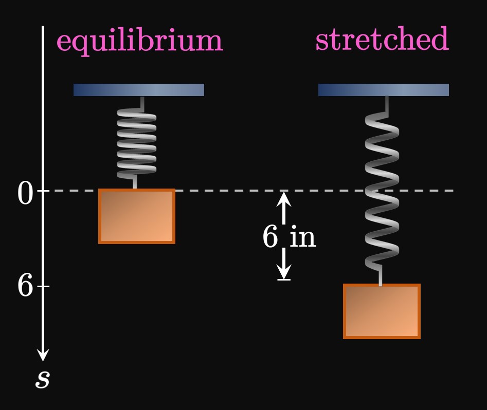
Velocity and Acceleration Velocity \(v(t)\) is the derivative of \(s(t) \col\) \[v(t) = \deriv{}{t} \par{6 \cos t} = \boxed{-6 \sin t}\] Acceleration \(a(t)\) is the derivative of \(v(t) \col\) \[a(t) = \deriv{}{t} \par{-6 \sin t} = \boxed{-6 \cos t}\] Note that \(a(t) = -s(t).\)
Analysis Because \(a(t) = -s(t),\) we notice that at the equilibrium position, \(s(t) = 0\) and so \(a(t) = 0.\) This equation also asserts that the magnitude of the block's acceleration is greatest at the highest and lowest points of its motion (since \(s\) is greatest at these points). Conversely, the object's speed function is given by \(\abs{v(t)}\) \(= 6 \abs{\sin t},\) which is \(0\) when \(t = 0.\) The speed is maximized when \(\abs{\sin t} = 1,\) which occurs when \(\cos t = 0.\) Hence, the block's speed is greatest as it passes through equilibrium but is \(0\) at the highest and lowest points.
Power Rule The Power Rule enables us to differentiate power functions. If \(n\) is any real number, then the Power Rule gives \begin{equation} \deriv{}{x} \par{x^n} = nx^{n - 1} \pd \eqlabel{eq:power-rule} \end{equation} In words, to differentiate a power function we multiply by the power and then subtract \(1\) from the exponent. This formula is applicable only when the base is a variable and the power is a constant.
Equations of Tangent Lines and Normal Lines If \(f\) is differentiable at \(a,\) then the line tangent to the curve \(y = f(x)\) at \(x = a\) is given by the equation \begin{equation} y - f(a) = f'(a) \par{x - a} \pd \eqlabel{eq:tan-line} \end{equation} A normal line intersects a curve at an angle of \(90 \degree\) and is perpendicular to a tangent line. The line normal to the curve \(y = f(x)\) at \(x = a\) is given by the equation \begin{equation} y - f(a) = -\frac{1}{f'(a)}(x - a) \pd \eqlabel{eq:normal-line} \end{equation}
Differentiating \(e^x\) An exponential function has a variable power. Euler's number \((e \approx 2.718)\) is the number for which \begin{equation} \lim_{h \to 0} \frac{e^h - 1}{h} = 1 \pd \eqlabel{eq:e-lim} \end{equation} Consequently, this limit yields \begin{equation} \deriv{}{x} \par{e^x} = e^x \pd \eqlabel{eq:deriv-e^x} \end{equation}
Derivatives of Sine and Cosine The derivative of sine is cosine, and the derivative of cosine is negative sine: \begin{align} \deriv{}{x} \par{\sin x} &= \cos x \eqlabel{eq:deriv-sin} \nl \deriv{}{x} \par{\cos x} &= - \sin x \eqlabel{eq:deriv-cos} \pd \end{align}