7.6: Probability
Probability measures the chance that an event occurs. Outcomes of dice rolling, card selection, and basketball shots are examples of discrete probabilities because they have a finite number of possible outcomes. In calculus we work with continuous probabilities, in which a number can take on any value. A store might want to determine the probability that a customer waits in line for more than \(2\) minutes, or a doctor might want to know the probability that her patient has a blood pressure above \(130 \un{mm Hg}.\) We discuss the following topics:
- Probability Density Functions
- Exponential Probability Density Functions
- Mean of a Probability Density Function
- Normal Distribution
Probability Density Functions
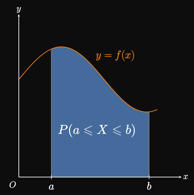
Let \(X\) denote a continuous random variable, meaning \(X\) is randomly assigned any number. The probability that the value of \(X\) lands between the numbers \(a\) and \(b\) is written as \[P(a \leq X \leq b) \pd\] Suppose that a continuous random variable \(X\) has a probability density function \(f,\) defined such that \(f(x) \geq 0\) and \begin{equation} P(a \leq X \leq b) = \int_a^b f(x) \di x \pd \label{eq:P-int} \end{equation} In words, to calculate the probability that \(X\) is between the numbers \(a\) and \(b,\) we find the area under the curve \(y = f(x)\) from \(x = a\) to \(x = b.\) (See Figure 1.) Because probabilities are measured from \(0\) to \(1,\) the total probability from \(x = -\infty\) to \(x = \infty\) must accumulate to \(1 \col\) \begin{equation} \int_{-\infty}^\infty f(x) \di x = 1 \pd \label{eq:prob-1} \end{equation} For a continuous random variable, we value probability density functions for the area under them; the particular values they output have little use to us.
- Verify that \(f\) is a probability density function.
- Find and interpret \(P(0 \leq X \leq 1/4).\)
- Observe that \(f(x) \geq 0\) for all \(x.\) The area under \(f\) is \(0\) for all \(x\) outside the interval \([0, 1],\) so \[ \ba \int_{-\infty}^{\infty} f(x) \di x &= \int_0^1 6x(1 - x) \di x \nl &= \par{3x^2 - 2x^3} \intEval_{0}^1 \nl &= 1 \pd \ea \] Since \(\int_{-\infty}^{\infty} f(x) \di x = 1,\) \(\eqrefer{eq:prob-1}\) is satisfied and so \(f(x)\) is a probability density function.
- Using \(\eqref{eq:P-int},\) the probability \(P(0 \leq X \leq 1/4)\) is given by integrating \(f(x)\) from \(x = 0\) to \(x = 1/4 \col\) \[ \ba P(0 \leq X \leq 1/4) &= \int_0^{1/4} 6x(1 - x) \di x \nl &= \par{3x^2 - 2x^3} \intEval_{0}^{1/4} \nl &= \parbr{3 \par{\tfrac{1}{4}}^2 - 2 \par{\tfrac{1}{4}}^3} - 0 \nl &= \boxed{\tfrac{5}{32}} \approx 0.156 \pd \ea \] Thus, under the distribution \(y = f(x),\) the probability of any number \(X\) residing between \(0\) and \(1/4\) is \(0.156,\) or \(15.6\%.\)
Exponential Probability Density Functions
Exponential decay functions are excellent probability density functions for phenomena such as waiting times and equipment longevity. Consider the following examples: At the checkout counter, you'll likely be helped within a few minutes, whereas long wait times are rarer. Likewise, among people who call into a support center, few customers are willing to wait for a long time. And a light bulb is unlikely to function for much longer than its expected lifespan. To derive a general probability density function \(f\) for such models, we let \(t\) be time (in any unit) such that \(f(t) = 0\) for \(t \lt 0.\) (You cannot be helped before you enter the line.) We have, for \(k \gt 0,\) \[ f(t) = \bc 0 & t \lt 0 \nl Ce^{-kt} & t \geq 0 \pd \ec \] Let's derive an expression for the area under the curve \(y = f(t).\) Clearly, the area under \(f\) over \(t\) in \((-\infty, 0)\) is \(0.\) Thus, we evaluate the improper integral (using the methods of Section 6.5) as follows: \[ \ba \int_{-\infty}^\infty f(t) \di t &= \int_0^\infty Ce^{-kt} \di t \nl &= \lim_{b \to \infty} \int_0^b Ce^{-kt} \di t \nl &= \frac{C}{-k} \lim_{b \to \infty} \par{e^{-kt}} \intEval_0^b \nl &= \frac{C}{-k} \par{0 - 1} \nl &= \frac{C}{k} \pd \ea \] By \(\eqref{eq:prob-1},\) \(\int_{-\infty}^\infty f(t) \di t\) must equal \(1.\) So \(C/k = 1,\) meaning \(C = k.\) Accordingly, all exponential decay functions are of the form \begin{equation} f(t) = \bc 0 & t \lt 0 \nl ke^{-kt} & t \geq 0 \pd \ec \label{eq:exp-density} \end{equation} (See Figure 2.) If \(C \ne k,\) then \(\eqref{eq:prob-1}\) is not satisfied and so \(f(t)\) cannot be a probability density function.

- Determine an exponential probability density function to model the wait times of customers at the checkout line.
- Calculate the probability that a customer is helped within \(5\) minutes.
- What is the probability that a customer waits more than \(5\) minutes for checkout?
- By \(\eqref{eq:exp-density},\) we model the wait times using the exponential decay function \[ f(t) = \bc 0 & t \lt 0 \nl ke^{-kt} & t \geq 0 \cma \ec \] where \(t\) is the time (in minutes) that a customer waits. Our goal is to solve for \(k.\) Since \(80\%\) of customers are helped at the checkout counter within \(2\) minutes, we have \(\int_0^2 f(t) \di t = 0.8.\) We see \[ \ba \int_0^2 ke^{-kt} \di t &= 0.8 \nl \frac{k}{-k} e^{-kt} \intEval_0^2 &= 0.8 \nl e^0 - e^{-2k} &= 0.8 \nl \implies k &= -\tfrac{1}{2} \ln 0.2 \approx 0.805 \pd \ea \] Hence, the exponential probability density function is \[ f(t) = \boxed{ \bc 0 & t \lt 0 \nl 0.805e^{-0.805t} & t \geq 0 \ec} \]
- Let \(T\) be the time a customer waits in line. The requested probability is \(P(0 \leq T \leq 5),\) whose value is given by the area under \(y = f(t)\) from \(0 \leq t \leq 5.\) By \(\eqref{eq:P-int},\) we have \[ \ba P(0 \leq T \leq 5) &= \int_0^5 0.805e^{-0.805t} \di t \nl &= \frac{0.805}{-0.805} e^{-0.805t} \intEval_0^5 \nl &= e^{0} - e^{-0.805(5)} \nl &\approx \boxed{0.982} = 98.2 \% \pd \ea \]
- If a customer waits in line for \(T\) minutes, then the probability of a wait longer than \(5\) minutes is given by \(P(T \gt 5).\) We see \[ P(T \gt 5) = \int_5^\infty f(t) \di t \pd \] Instead of computing the improper integral, we recognize that \(\int_0^\infty f(t) \di t = 1.\) Since the improper integral converges, it's easier to compute \(P(T \gt 5)\) by using the result from part (b) as follows: \[ \ba \int_0^\infty f(t) \di t &= \int_0^5 f(t) \di t + \int_5^\infty f(t) \di t \nl \implies \int_5^\infty f(t) \di t &= \int_0^\infty f(t) \di t - \int_0^5 f(t) \di t \nl &= 1 - 0.982 \nl &= \boxed{0.018} = 1.8 \% \pd \ea \]
Mean of a Probability Density Function
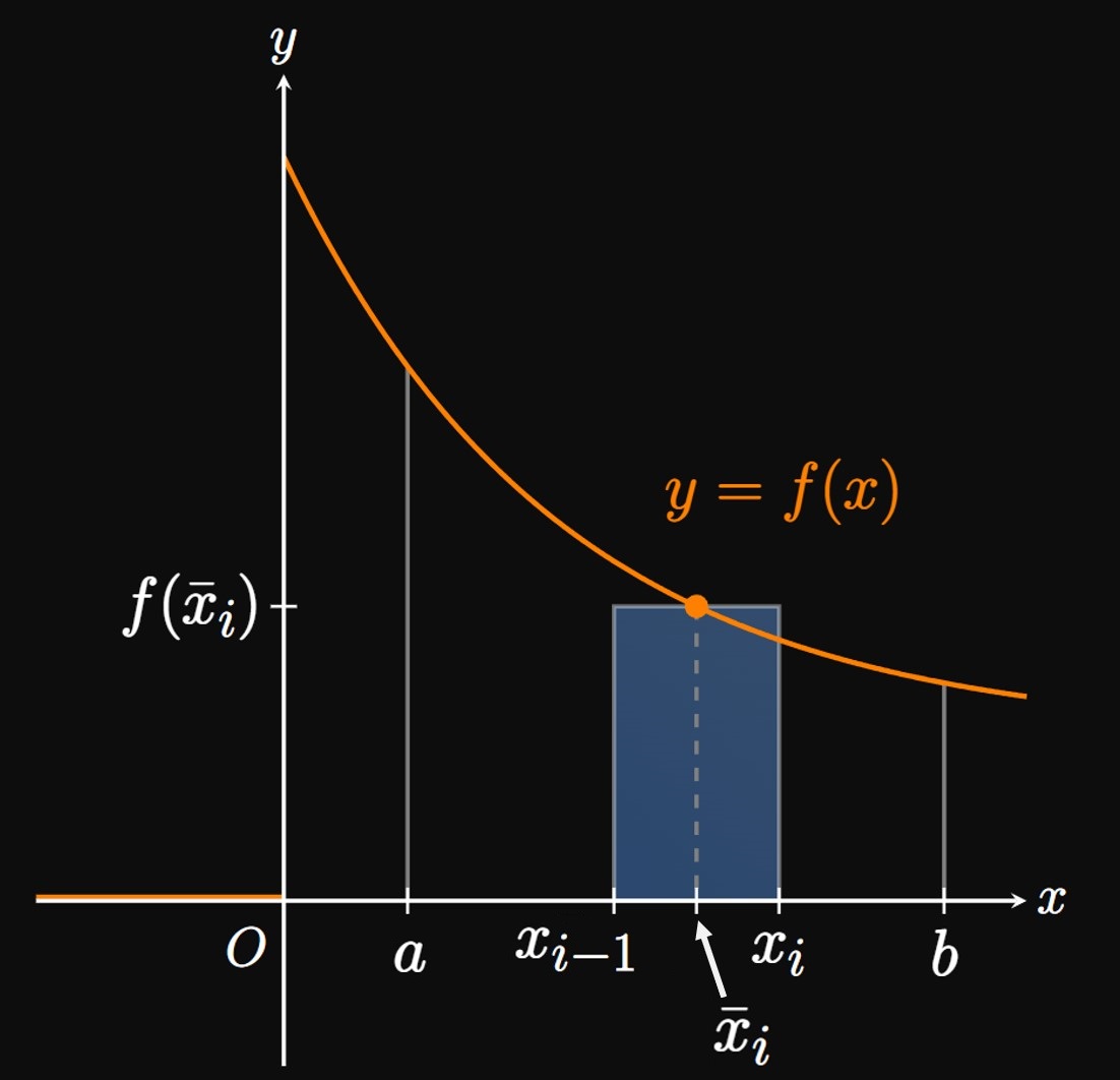
In a store or call center, it's imperative to know the average time a customer waits. Similarly, an equipment manufacturer must know how long a piece of equipment tends to last. These applications motivate the calculation of the mean of a probability density function—the long-run average value of a random variable \(X.\) Let \(y = f(x)\) be a probability density function. Suppose that \(N\) numbers are chosen in the interval \([a, b];\) we want to determine the sum of these \(N\) numbers. We split the interval \([a, b]\) into \(n\) subintervals; consider one subinterval from \(x_{i - 1}\) to \(x_i.\) If \(\overline{x}_i\) is the midpoint of these two numbers, then we assert the following: As we pick more and more numbers between \(x_{i - 1}\) and \(x_i,\) then the average of these numbers will approach \(\overline{x}_i.\) The probability of picking a number in \([a, b]\) and having it land in \([x_{i - 1}, x_i]\) is approximately \(f \par{\overline{x}_i} \Delta x,\) which is the area of the approximating rectangle in Figure 3. Accordingly, we estimate that the number of values landing in \([x_{i - 1}, x_i]\) is \(N f \par{\overline{x}_i} \Delta x.\) Each value is approximately \(\overline{x}_i,\) so the sum of these numbers is roughly \[N \, \overline{x}_i f \par{\overline{x}_i} \Delta x \pd\] To get the sum of all \(N\) numbers (across all \(n\) subintervals), we add the sums of the numbers in all \(n\) subintervals: \[\sum_{i = 1}^n N \, \overline{x}_i f \par{\overline{x}_i} \Delta x \pd\] This form is a Riemann sum for \(x f(x).\) We make each subinterval infinitely small by letting \(n \to \infty\) and \(\Delta x \to 0,\) so the limiting value of this Riemann sum is \[\int_a^b N x f(x) \di x \pd\] This is the sum of all \(N\) numbers, so we divide by \(N\) to get the mean \(\mu\) (mu): \[\mu = \int_a^b x f(x) \di x \pd\] More generally, the mean of a probability density function \(f(x)\) is given by \begin{equation} \mu = \int_{-\infty}^\infty x f(x) \di x \pd \label{eq:avg-X} \end{equation} This formula asserts that if we choose many values of the continuous random variable \(X,\) then the long-run average of \(X\) will be \(\mu.\) Observe that because \(\eqref{eq:avg-X}\) contains an extra term \(x\) in the integrand, the integral does not measure a probability; do not confuse it with \(\eqref{eq:prob-1}.\)
Since the mean of an exponential probability density function is \(\mu = 1/k\) (from Example 3), we can rewrite the probability density function in \(\eqref{eq:exp-density}\) as \begin{equation} f(t) = \bc 0 & t \lt 0 \nl \dfrac{e^{-t/\mu}}{\mu} & t \geq 0 \pd \ec \label{eq:prob-density-mu} \end{equation} This form is useful if we know the average waiting time \(\mu.\)
Normal Distribution
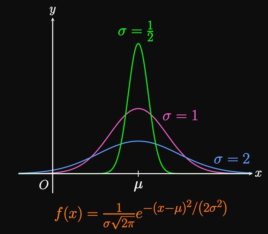
For centuries, statisticians have noticed a peculiar finding in homogeneous populations: Phenomena such as intelligence scores, test results, and heights are often distributed symmetrically around a central peak, resembling a bell curve. Specifically, a random variable \(X\) in these scenarios follows a Normal distribution, whose probability density function is \begin{equation} f(x) = \frac{1}{\sigma \sqrt{2 \pi}} \, e^{-(x - \mu)^2/\par{2 \sigma^2}} \pd \label{eq:normal-pdf} \end{equation} This is one of the most important distributions in statistics, with many applications in inferential statistics, probability calculations, and the natural sciences. It turns out that the factor \(1/\par{\sigma \sqrt{2 \pi}}\) is needed to satisfy \(\int_{-\infty}^\infty f(x) \di x = 1,\) thus enabling \(f\) to be a probability density function. The mean of this function is \(\mu,\) and the parameter \(\sigma\) (sigma) is called the standard deviation, a measure of variation in the values of \(X.\) Low values of \(\sigma\) imply little spread, meaning the graph of \(y = f(x)\) tends to be clustered around the mean. Conversely, high values of \(\sigma\) indicate large spread, so the graph of \(y = f(x)\) is more flattened around the mean. (See Figure 4.)
The 68–95–99.7 Rule Unfortunately, the function in \(\eqref{eq:normal-pdf}\) has no elementary antiderivative. We must instead use methods such as Riemann sums or Simpson's Rule to approximate integrals with this function. Using such methods produces the following results: \[ \ba \int_{\mu -\sigma}^{\mu + \sigma} \frac{1}{\sigma \sqrt{2 \pi}} \, e^{-(x - \mu)^2/\par{2 \sigma^2}} \di x &\approx 0.68 \cma\nl \int_{\mu -2\sigma}^{\mu + 2\sigma} \frac{1}{\sigma \sqrt{2 \pi}} \, e^{-(x - \mu)^2/\par{2 \sigma^2}} \di x &\approx 0.95 \cma \nl \int_{\mu -3\sigma}^{\mu + 3\sigma} \frac{1}{\sigma \sqrt{2 \pi}} \, e^{-(x - \mu)^2/\par{2 \sigma^2}} \di x &\approx 0.997 \pd \ea \] These results are summarized by the 68–95–99.7 Rule (also called the Empirical Rule), which says that about \(68\%\) of the data lie within \(1\) standard deviation of the mean, about \(95\%\) of the data lie within \(2\) standard deviations of the mean, and about \(99.7\%\) of the data lie within \(3\) standard deviations of the mean. Hence, it is very rare for a random variable \(X\) to lie more than \(3\) standard deviations away from the mean. We use the 68–95–99.7 Rule to estimate probabilities in our heads, as well as how likely an outcome is to occur. In general, statisticians consider significant any value of \(X\) located more than \(2\) standard deviations away from the mean, which has only a \(5\%\) chance to occur.

The Intelligence Quotient A measure of intelligence is the Intelligence Quotient (IQ), whose scores are Normally distributed with a mean of \(\mu = 100\) and a standard deviation of \(\sigma = 15.\) Substituting these parameters into \(\eqref{eq:normal-pdf}\) gives a probability density function for IQ scores to be \begin{equation} f(x) = \normalPdf{100}{15}{x} \pd \label{eq:iq} \end{equation} (See Figure 5.) By the 68–95–99.7 Rule, we conclude the following:
- About \(68 \%\) of people have IQs between \(85\) and \(115.\)
- About \(95 \%\) of people have IQs between \(70\) and \(130.\)
- About \(99.7 \%\) of people have IQs between \(55\) and \(145.\)
- Derive the probability density function for this model.
- In a sample of \(1000\) randomly selected women, approximately how many have a height between \(62\) inches and \(67\) inches?
- What is the probability that a woman is \(68\) inches or taller?
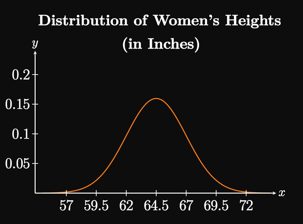
- The mean of this distribution is \(\mu = 64.5,\) with a standard deviation of \(\sigma = 2.5.\) Substituting these values into \(\eqref{eq:normal-pdf}\) gives the probability density function \[f(x) = \boxed{\normalPdf{64.5}{2.5}{x}}\]
- The value \(62\) is \(1\) standard deviation lower than the mean, and the value \(67\) is \(1\) standard deviation higher than the mean. By the 68–95–99.7 Rule, in a Normal distribution approximately \(68\%\) of values lie within one standard deviation of the mean. So we estimate that, out of \(1000\) women, the number whose heights are between \(62\) and \(67\) inches is \[1000 \times 0.68 = \boxed{680}\]
- The probability that a woman is taller than \(68\) inches is given by integrating the probability density function \(f(x)\) from \(x = 68\) to \(x = \infty.\) But to avoid the improper integral, we instead use a sufficiently large number as an upper bound—for example, \(x = 90,\) which is more than \(10\) standard deviations away from the mean and is therefore extremely rare. Using numerical methods or a calculator, we see \[ \ba P(X \geq 68) &\approx \int_{68}^{90} \normalPdf{64.5}{2.5}{x} \di x \nl &\approx \boxed{0.0808} = 8.08 \% \pd \ea \] Thus, about \(8.08\%\) of women in the United States are \(68\) inches or taller.
Probability Density Functions If \(X\) is a continuous random variable (that is, \(X\) is randomly assigned any number) and \(f(x)\) is a probability density function, then \(f(x) \geq 0\) and \(\int_{-\infty}^\infty f(x) \di x = 1,\) and the probability that \(X\) lies between \(a\) and \(b\) is \begin{equation} P(a \leq X \leq b) = \int_a^b f(x) \di x \pd \eqlabel{eq:P-int} \end{equation} For a continuous random variable, we use probability density functions for the area under them; the particular values they output have little use to us.
Exponential Probability Density Functions We often use exponential decay functions as probability density functions for phenomena such as waiting times and equipment longevity. If \(k \gt 0,\) then an exponential probability density function takes the form \begin{equation} f(t) = \bc 0 & t \lt 0 \nl ke^{-kt} & t \geq 0 \pd \ec \eqlabel{eq:exp-density} \end{equation}
Mean of a Probability Density Function If \(f\) is a probability density function, then the mean of a probability density function is given by \begin{equation} \mu = \int_{-\infty}^\infty x f(x) \di x \pd \eqlabel{eq:avg-X} \end{equation} The number \(\mu\) is the long-run average of the random variable \(X;\) as we select more and more values of \(X,\) the average of these numbers becomes \(\mu.\) An exponential probability density function has a mean of \(\mu = 1/k,\) so we can write the density function as \begin{equation} f(t) = \bc 0 & t \lt 0 \nl \dfrac{e^{-t/\mu}}{\mu} & t \geq 0 \pd \ec \eqlabel{eq:prob-density-mu} \end{equation} This form is useful if \(\mu\) is measurable (for example, the average time a customer waits in line).
Normal Distribution A Normal distribution has a probability density function given by \begin{equation} f(x) = \frac{1}{\sigma \sqrt{2 \pi}} \, e^{-(x - \mu)^2/\par{2 \sigma^2}} \cma \eqlabel{eq:normal-pdf} \end{equation} where \(\mu\) is the mean of the probability density function and \(\sigma\) is the standard deviation, a measure of variation. The graph of \(y = f(x)\) is symmetrical about a central peak and is a bell-shaped curve. The 68–95–99.7 Rule (also called the Empirical Rule), enables us to estimate probabilities within a Normal distribution, as follows:
- About \(68\%\) of the data lie within \(1\) standard deviation of the mean.
- About \(95\%\) of the data lie within \(2\) standard deviations of the mean.
- About \(99.7\%\) of the data lie within \(3\) standard deviations of the mean. It is very rare for a random variable \(X\) to lie more than \(3\) standard deviations away from the mean.