9.2: Differentiating and Integrating Parametric Functions
When we ventured into applications of integration, we saw how important derivatives are. In this section we investigate the utility of parametric functions to model a variety of situations, so in this section we merge these topics. We discuss the following:
Differentiating Parametric Functions
How do we calculate the slope of a graph parameterized by \(x = f(t)\) and \(y = g(t) \ques\) If \(f\) and \(g\) are differentiable functions, and \(y\) is differentiable with respect to \(x,\) then the Chain Rule (from Section 2.4) states \[\deriv{y}{t} = \deriv{y}{x} \deriv{x}{t} \pd\] Dividing both sides by \(\textderiv{x}{t}\) (assuming it is nonzero) gives \begin{equation} \deriv{y}{x} = \frac{\textderiv{y}{t}}{\textderiv{x}{t}} \pd \label{eq:dy/dx} \end{equation} We can also write \(\textderiv{y}{x} = g'(t)/f'(t).\) \(\eqrefer{eq:dy/dx}\) permits us to calculate slopes to a graph without eliminating the parameter \(t;\) that is, \(\textderiv{y}{x}\) is a function of \(t.\) In words, we divide the derivative of \(y\) with respect to \(t\) by the derivative of \(x\) with respect to \(t.\) This form is easy to remember if you think of canceling the \(\dd t\)'s.
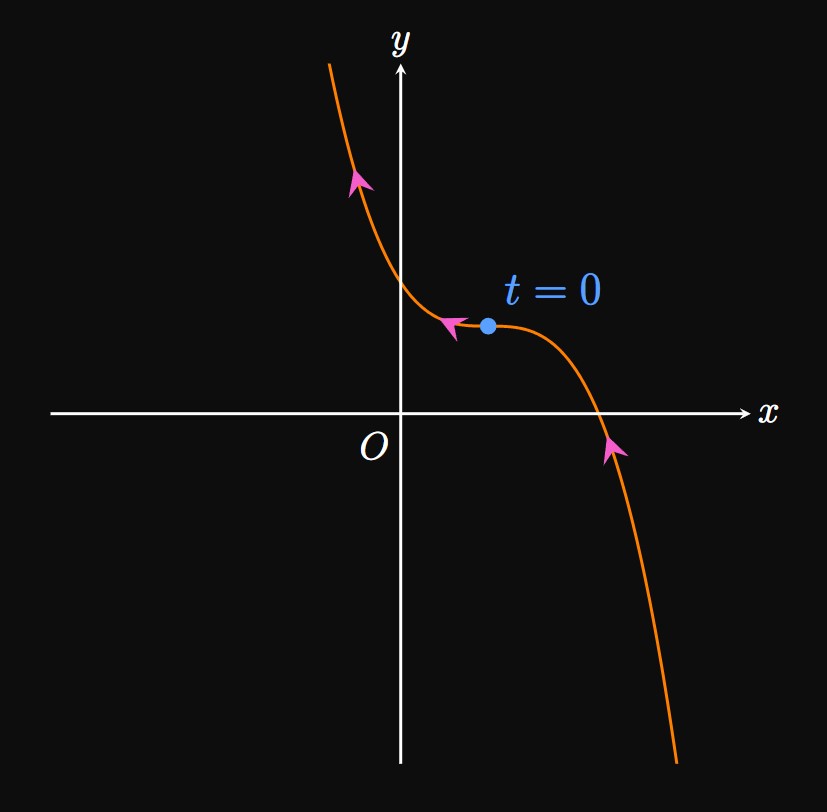
- Write an equation of the line tangent to the graph at \(t = 2.\)
- Locate all horizontal tangents and vertical tangents to the graph.
- The slope is given by \(\textderiv{y}{x}\) when \(t = 2.\) We first compute \(\textderiv{x}{t}\) and \(\textderiv{y}{t} \col\) \[\deriv{x}{t} = 4t - 1 \lspace \deriv{y}{t} = 6 - 6t \pd\] Then by \(\eqrefer{eq:dy/dx},\) we see \[\deriv{y}{x} \intEval_{t = 2} = \frac{6 - 6(2)}{4(2) - 1} = -\frac{6}{7} \pd\] When \(t = 2,\) \[x = 2(2)^2 - 2 = 6 \and y = 6(2) - 3(2)^2 = 0 \pd\] Thus, an equation of the tangent line is \[y - 0 = -\tfrac{6}{7}(x - 6) \implies \boxed{y = -\tfrac{6}{7}(x - 6)}\]
-
The graph has a horizontal tangent when \(\textderiv{y}{x} = 0,\) which occurs when \(\textderiv{y}{t} = 0\) but \(\textderiv{x}{t} \ne 0.\) We find \[\deriv{y}{t} = 6 - 6t = 0 \implies t = 1 \pd\] At \(t = 1,\) \(\textderiv{x}{t}\) is nonzero. Thus, the graph has a horizontal tangent when \(t = 1,\) which corresponds to the point \((1, 3).\)
Conversely, the graph has a vertical tangent when \(\textderiv{x}{t} = 0\) but \(\textderiv{y}{t} \ne 0.\) We see \[\deriv{x}{t} = 4t - 1 = 0 \implies t = \tfrac{1}{4} \pd\] At this value, \(\textderiv{y}{t} \ne 0.\) The graph therefore has a vertical tangent when \(t = 1/4,\) or at the point \((-1/8, 21/16).\)

Higher-Order Derivatives To determine higher-order derivatives, we use \(\eqrefer{eq:dy/dx}\) repeatedly. We replace \(y\) (a function of \(t\)) with \(\textderiv{y}{x}\) (another function of \(t\)) to attain \begin{equation} \deriv{^2 y}{x^2} = \deriv{}{x} \par{\deriv{y}{x}} = \frac{\ds \deriv{}{t}\left(\deriv{y}{x}\right)}{\textderiv{x}{t}} \pd \label{eq:2-dy/dx} \end{equation} For the general, \(n\)th derivative we replace \(y\) with \(\textderiv{^{n - 1} y}{x^{n - 1}}\) to get \begin{equation} \deriv{^n y}{x^n} = \deriv{}{x} \par{\deriv{^{n - 1}y}{x^{n - 1}}} = \frac{\ds \deriv{}{t}\left(\deriv{^{n - 1}y}{x^{n - 1}}\right)}{\textderiv{x}{t}} \pd \label{eq:n-dy/dx} \end{equation}

Areas with Parametric Curves
Integrating Vertically In Cartesian coordinates, the area bounded by a curve and the \(x\)-axis from \(x = a\) to \(x = b\) is \(\int_a^b y \di x.\) Recall that the integral is positive if \(y \gt 0\) and negative if \(y \lt 0.\) We now consider the area under a curve defined parametrically by \begin{equation} x = f(t) \lspace y = g(t) \cma \label{eq:par-eqs} \end{equation} where \(f\) and \(g\) are both differentiable. Our goal is to use the Substitution Rule (from Section 4.4) to convert \(\int_a^b y \di x\) to be an integral in terms of \(t.\) From \(\eqref{eq:par-eqs}\) we see \(\textderiv{x}{t} = f'(t),\) or \(\dd x = f'(t) \di t.\) To express the bounds of the integral in terms of \(t,\) let \(t_a\) and \(t_b\) be values of \(t\) such that \(f(t_a) = a\) and \(f(t_b) = b.\) Assuming the parametric curve is traced out once over \(t_a \leq t \leq t_b,\) the integral \(\int_a^b y \di x\) becomes \begin{equation} \int_{t_a}^{t_b} g(t) f'(t) \di t \pd \label{eq:area-x} \end{equation}
Integrating Horizontally The area between a curve and the \(y\)-axis from \(y = c\) to \(y = d\) is \(\int_c^d x \di y,\) which is positive if \(x \gt 0\) and negative if \(x \lt 0.\) In \(\eqref{eq:par-eqs}\) we have \(\textderiv{y}{t} = g'(t),\) or \(\dd y = g'(t) \di t.\) Let \(t_c\) and \(t_d\) satisfy \(g(t_c) = c\) and \(g(t_d) = d.\) The integral \(\int_c^d x \di y\) therefore becomes \begin{equation} \int_{t_c}^{t_d} f(t) g'(t) \di t \pd \label{eq:area-y} \end{equation}


Differentiating Parametric Functions If \(f\) and \(g\) are differentiable functions and \(y\) is differentiable with respect to \(x,\) then \begin{equation} \deriv{y}{x} = \frac{\textderiv{y}{t}}{\textderiv{x}{t}} \pd \eqlabel{eq:dy/dx} \end{equation} In this form, \(\textderiv{y}{x}\) is a function of \(t,\) enabling us to find slopes of a parametric curve without eliminating the parameter. The higher-order derivatives are as follows: The second derivative is \begin{equation} \deriv{^2 y}{x^2} = \frac{\ds \deriv{}{t}\left(\deriv{y}{x}\right)}{\textderiv{x}{t}} \pd \eqlabel{eq:2-dy/dx} \end{equation} The general, \(n\)th derivative is \begin{equation} \deriv{^n y}{x^n} = \frac{\ds \deriv{}{t}\left(\deriv{^{n - 1}y}{x^{n - 1}}\right)}{\textderiv{x}{t}} \pd \eqlabel{eq:n-dy/dx} \end{equation}
Areas with Parametric Curves Consider a curve defined parametrically by \(x = f(t)\) and \(y = g(t).\) The area bounded by the curve and the \(x\)-axis from \(x = a\) to \(x = b,\) where \(f(t_a) = a\) and \(f(t_b) = b,\) is \begin{equation} \int_{t_a}^{t_b} g(t) f'(t) \di t \pd \eqlabel{eq:area-x} \end{equation} The area bounded by the curve and the \(y\)-axis from \(y = c\) to \(y = d,\) where \(g(t_c) = c\) and \(g(t_d) = d,\) is \begin{equation} \int_{t_c}^{t_d} f(t) g'(t) \di t \pd \eqlabel{eq:area-y} \end{equation}
