9.1: Parametric Equations

So far, we have primarily modeled graphs using the form \(y = f(x).\) But these models cannot express curves that fail the Vertical Line Test—that is, curves that cannot be represented by functions. For example, it's impossible to describe the full circle \(x^2 + y^2 = r^2\) using the form \(y = f(x);\) solving for \(y\) gives either \[y = \sqrt{r^2 - x^2} \or y = - \sqrt{r^2 - x^2} \cma\] each of which represents a semicircle. In this section we learn to represent curves using parametric equations, in which we describe \(x\) and \(y\) independently by using a third variable \(t.\) We will learn convenient tools to model the entire circle \(x^2 + y^2 = r^2\) and present applications of parametric functions. We discuss the following topics:

• Defining a Parametric Curve
• Eliminating the Parameter
• Parameterizing Circles
• Parameterizing Ellipses
• The Cycloid
• Projectile Motion

Defining a Parametric Curve

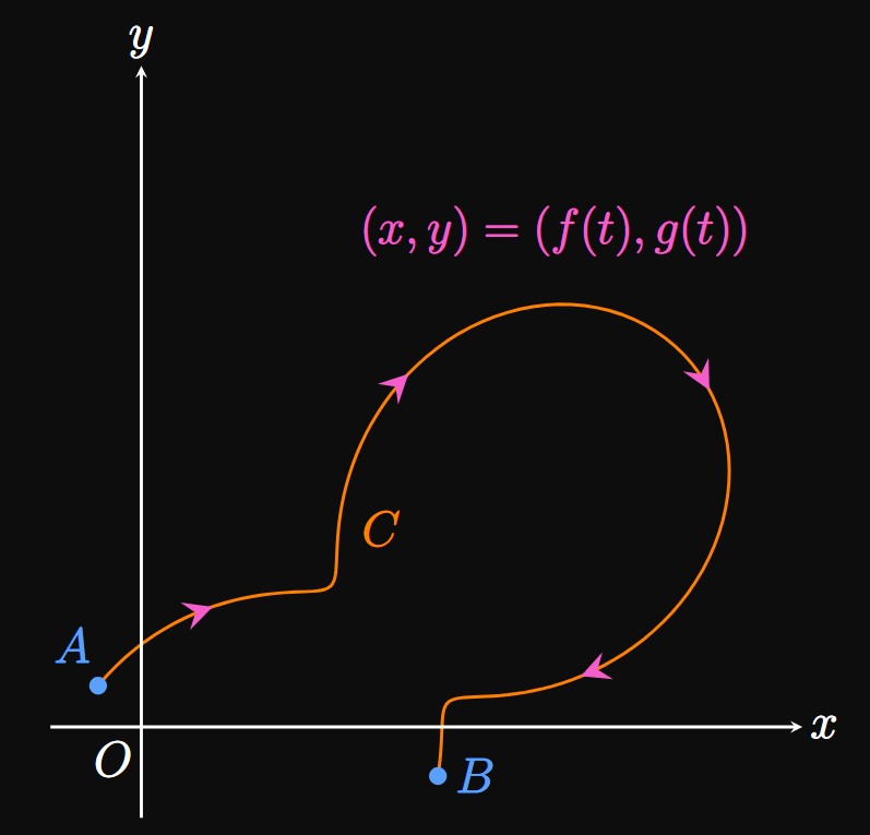
A curve can be described by a set of parametric equations \[x = f(t) \lspace y = g(t) \cma\] which give the graph's \(x\)- and \(y\)-coordinates at any value \(t,\) called a parameter. As \(t\) changes, the point \((f(t), g(t))\) varies and traces out a curve in the \(xy\)-plane. In Figure 1, the curve \(C\) is parameterized by the equations \(x = f(t)\) and \(y = g(t)\) because for some number \(t,\) the functions \(f\) and \(g\) give a point on the graph. Arrowheads represent the direction in which the curve is traced as \(t\) increases. We may limit the interval of \(t\) to confine a curve to be a certain shape. Point \(A\) is the initial point, and point \(B\) is the terminal point.

Introducing the parameter \(t\) enables \(x\) and \(y\) to vary independently of each other. Think of the parameter as a third variable that helps us express \(x\) and \(y\) without needing to relate them. (In some cases, it's difficult—even impossible—to write an equation to link \(x\) and \(y.\)) In many applications, we view \(t\) as time: If a particle moves along a curve, then its \(x\)- and \(y\)-coordinates are changing with time \(t.\) Later in this section, we will use parametric equations to describe Projectile Motion. But \(t\) doesn't need to be time; we can have negative values of \(t,\) and we could choose another letter in place of \(t.\)

Let's plot some points on the graph. A table of selected values of \(t,\) along with their corresponding values of \(x\) and \(y,\) is shown below.

\(t\)	\(x\)	\(y\)
\(-3\)	\(-5\)	\(5\)
\(-2\)	\(-4\)	\(0\)
\(-1\)	\(-3\)	\(-3\)
\(0\)	\(-2\)	\(-4\)
\(1\)	\(-1\)	\(-3\)
\(2\)	\(0\)	\(0\)
\(3\)	\(1\)	\(5\)

Plotting these points gives the parabola in Figure 2. Imagine a particle moving along the curve; as \(t\) is increased, the particle's path traces out the parabola. Labeled points appear in equal time intervals but not necessarily equal distances. For example, when \(t = 0\) the particle moves the slowest, but as \(t\) is increased the particle begins to speed up (and thus cover more distance). Since we have no limitation to the values of \(t,\) the parametric equations \(x = t - 2\) and \(y = t^2 - 4\) model an entire parabola.

Eliminating the Parameter

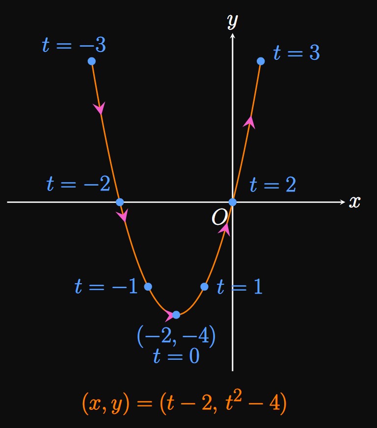
In Example 1, the parametric equations trace out a parabola. Yet we cannot rely on tables to show the shapes of parametric curves: Just as with graphs given by Cartesian equations (which directly relate \(x\) and \(y\)), tables often miss key features of graphs. For example, it's easy to miss the asymptotes of rational functions if we simply plot points. One could easily miss the vertical asymptote \(x = 0\) on the graph of \(y = 1/x.\) And rough sketches fail to provide precise values of interest, such as intercepts and extrema. Hence, we need a more formal route to verify the shape of a parametric curve, for which we eliminate the parameter.

Eliminating the parameter is the process by which we directly relate \(x\) and \(y\) using one equation without the parameter \(t.\) In other words, when we eliminate the parameter we write a Cartesian equation to represent a parametric curve. Imagine a curve defined by two parametric equations. Generally, from one parametric equation we want to solve for \(t\) in terms of \(x\) or \(y,\) and substitute this expression into the other parametric equation. In Example 1, which has the parametric equations \(x = t - 2\) and \(y = t^2 - 4,\) solving for \(t\) in the first parametric equation \((x = t - 2)\) yields \(t = x + 2.\) Then substituting this expression into the second parametric equation \((y = t^2 - 4)\) gives \[y = (x + 2)^2 - 4 \cma\] the Cartesian equation of a parabola with vertex \((-2, -4).\) In this form, \(x\) and \(y\) are related to each other by a single equation that doesn't contain \(t.\) Hence, the curve parameterized by \(x = t - 2\) and \(y = t^2 - 4\) can also be represented by \(y = (x + 2)^2 - 4.\)

When we eliminate the parameter in a set of parametric equations, we lose information about the direction of motion. In Example 1 as \(t\) is increased, the point \((x, y)\) moves from left to right along the parabola \(y = (x + 2)^2 - 4.\) But our Cartesian equation doesn't indicate this direction; it only models the parabola itself. If parametric equations represent a particle's motion, then upon eliminating the parameter we forfeit information about the particle's initial position and direction of motion. Hence, eliminating the parameter only provides us with the shape of the path.

When we eliminate the parameter, we relate \(x\) and \(y\) to each other using a single equation. The easiest procedure is as follows: Solving for \(t\) in the second parametric equation \((y = 2t)\) gives \(t = y/2,\) which we substitute into the first parametric equation \((x = 3 + 3 \sin t)\) to attain \[x = 3 + 3 \sin \par{\frac{y}{2}} \pd\] We now consider the endpoints of the interval \(-\pi \leq t \leq \pi \col\) When \(t = -\pi,\) \(x = 3\) and \(y = -2 \pi.\) When \(t = \pi,\) \(x = 3\) and \(y = 2 \pi.\) Thus, the curve is a sine graph confined to \(0 \leq x \leq 6\) and \(-2 \pi \leq y \leq 2 \pi.\) The initial point is \((3, -2\pi),\) and the terminal point is \((3, 2\pi).\) (See Figure 3.) In this example, writing parametric equations is useful since \(y\) cannot be defined as a function of \(x.\)

Sometimes we can eliminate the parameter without solving for \(t.\) Throughout this section, we will see that we can exploit trigonometric identities to directly relate \(x\) and \(y\) to each other.

Parameterizing Circles

We now return to the question at the beginning of this section: how do we represent a full circle using parametric functions? A circle doesn't extend indefinitely in the coordinate plane (unlike in Example 1, where the parabola is traced out forever). As the parameter \(t\) is made arbitrarily large, the points \((x, y)\) must repeat themselves. Therefore, to model a circle we need to use periodic functions.

By plotting some points, the curve resembles a circle. (Remember, however, that plotting points may not tell the full story.) To verify this shape, we eliminate the parameter by using the Pythagorean identity: \[x^2 + y^2 = \cos^2 t + \sin^2 t = 1 \pd\] Thus, the parametric equations produce the Unit Circle, whose Cartesian equation is \(x^2 + y^2 = 1.\) As \(t\) is increased from \(0,\) the point \((x, y)\) \(= (\cos t, \sin t)\) starts at \((1, 0)\) and rotates counterclockwise. The entire circle is traced once over the interval \(0 \leq t \leq 2 \pi;\) outside this interval, points stack on top of each other and so retrace the circle. In this special case, we can interpret \(t\) as the central angle of the Unit Circle. (See Figure 4.)

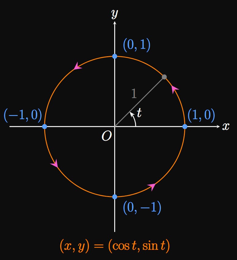
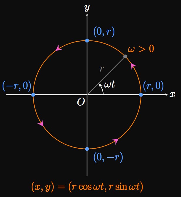
Circle Centered at the Origin Example 3 shows a parameterization of a Unit Circle centered at the origin. We now generalize the example to a circle of radius \(r\) centered at the origin, whose Cartesian equation is \(x^2 + y^2 = r^2.\) Consider the equations \(x = r \cos t\) and \(y = r \sin t.\) To eliminate the parameter, we exploit the Pythagorean identity to verify that \[ \ba x^2 + y^2 &= (r \cos t)^2 + (r \sin t)^2 \nl &= r^2 \, (\cos^2 t + \sin^2 t) \nl &= r^2 \pd \ea \] Hence, the parametric equations \(x = r \cos t\) and \(y = r \sin t\) satisfy \(x^2 + y^2 = r^2\) and so parametrize a circle of radius \(r.\) When \(t = 0,\) the point \((x, y)\) \(= (r \cos t, r \sin t)\) is at \((r, 0).\) Interestingly, the parametric equations \(x = r \sin t\) and \(y = r \cos t\) also trace out the same circle, although when \(t = 0\) the point \((x, y) =\) \((r \sin t, r \cos t)\) begins at \((0, r).\) Therefore, there are multiple ways to parameterize a curve—in fact, infinitely many ways. For example, the family of parametric equations \begin{equation} x = \pm r \cos \omega t \lspace y = \pm r \sin \omega t \label{eq:para-circle} \end{equation} represents a circle of radius \(r\) for any number \(\omega\) (omega), since the parametric equations satisfy \(x^2 + y^2 = r^2\) for any \(\omega.\) When \(t = 0,\) the curve traced out by \(\eqref{eq:para-circle}\) is at the point \((\pm r, 0).\) Figure 5 depicts the graph of \(x = r \cos \omega t\) and \(y = r \sin \omega t\) for a positive number \(\omega;\) when \(t = 0,\) the point \((x, y)\) is at \((r, 0).\) Conversely, the parametric equations \begin{equation} x = \pm r \sin \omega t \lspace y = \pm r \cos \omega t \label{eq:para-circle-2} \end{equation} parameterize the same circle of radius \(r,\) yet when \(t = 0\) the curve begins at \((0, r).\) Changing \(\omega\) varies the speed at which the circle is traced out: In \(\eqref{eq:para-circle}\) and \(\eqref{eq:para-circle-2},\) if \(\omega = 1\) then \(1\) radian is traced out if we increase \(t\) by \(1.\) The entire circle is therefore traced out in \(2 \pi\) time units. Likewise, if \(\omega = 2\) then \(2\) radians are traced out per increment of \(t\) by \(1,\) so the entire circle is traced out in \(\pi\) time units. For circles (and circles only), we interpret \(\abs{\omega}\)—called the angular frequency—as the number of radians traced out per time unit.

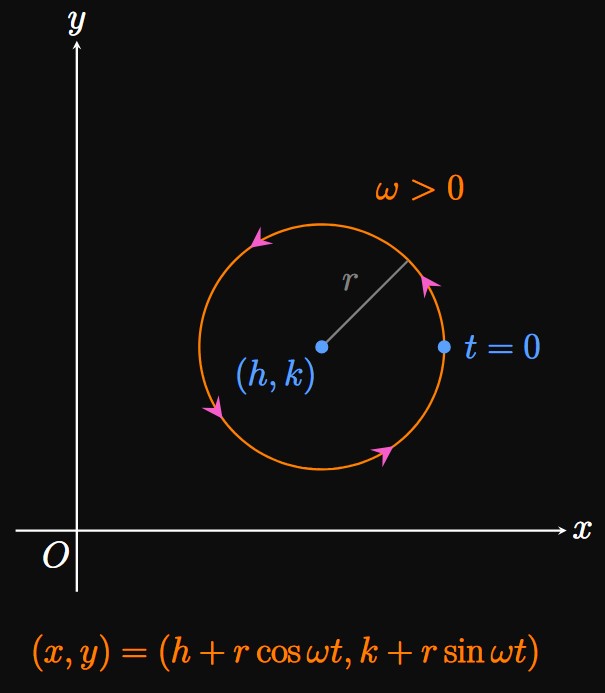
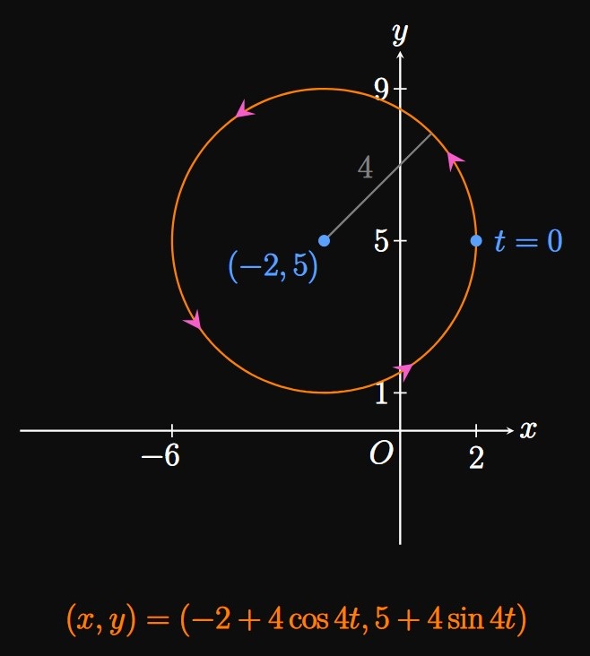
Circle Centered at Any Point A circle of radius \(r\) centered at some point \((h, k)\) is represented by the Cartesian equation \begin{equation} (x - h)^2 + (y - k)^2 = r^2 \pd \label{eq:cart-circle-h-k} \end{equation} To find parametric equations, we again exploit the Pythagorean identity: We want \(\eqrefer{eq:cart-circle-h-k}\) to match the form \((\pm r \cos \omega t)^2 + (\pm r \sin \omega t)^2 = r^2,\) so we let \begin{alignat}{2} x - h &= \pm r \cos \omega t \lspace y - \, &&k = \pm r \sin \omega t \nonumber \nl x &= h \pm r \cos \omega t \lspace &&y = k \pm r \sin \omega t \label{eq:para-circle-hk} \pd \end{alignat} Alternatively, we could analogize \(\eqrefer{eq:cart-circle-h-k}\) to \((\pm r \sin \omega t)^2 + (\pm r \cos \omega t)^2 = r^2,\) from which we attain \begin{alignat}{2} x - h &= \pm r \sin \omega t \lspace y - \, &&k = \pm r \cos \omega t \nonumber \nl x &= h \pm r \sin \omega t \lspace &&y = k \pm r \cos \omega t \label{eq:para-circle-hk-alt} \pd \end{alignat} The parametric equations of \(\eqref{eq:para-circle-hk}\) indicate that when \(t = 0,\) the point \((x, y)\) is at the farthest left or farthest right of the circle. For example, in Figure 6 the point \((x, y)\) is at \((h + r, k)\) when \(t = 0.\) By contrast, we use \(\eqref{eq:para-circle-hk-alt}\) to model a circle such that when \(t = 0\) the point \((x, y)\) is at the top or bottom of the circle.

When \(t = 0,\) the point \((x, y)\) is at the farthest right of the circle. From \(\eqref{eq:para-circle-hk},\) we parameterize the circle using the form \[x = -2 \pm 4 \cos \omega t \lspace y = 5 \pm 4 \sin \omega t\] for some number \(\omega.\) Because the circle is fully traced in \(\pi/2\) time units, as \(t\) increases by \(1\) the circle is traced out by \[\frac{2 \pi}{\pi/2} = 4 \un{rad} \pd\] Hence, \(\omega = 4\) and so our preliminary equations are \[x = -2 \pm 4 \cos 4t \lspace y = 5 \pm 4 \sin 4t \pd\] We now select whether to make the coefficients of the sinusoidal functions positive or negative. Since the circle is traced counterclockwise, \(x\) is decreasing and \(y\) is increasing as \(t\) increases from \(0.\) For positive \(t\) near \(0,\) the function \(x = -2 + 4 \cos 4 t\) is decreasing and the function \(y = 5 + 4 \sin 4t\) is increasing. The final equations are therefore \[\boxed{x = -2 + 4 \cos 4t} \and \boxed{y = 5 + 4 \sin 4t}\] (See Figure 7.)

Parameterizing Ellipses

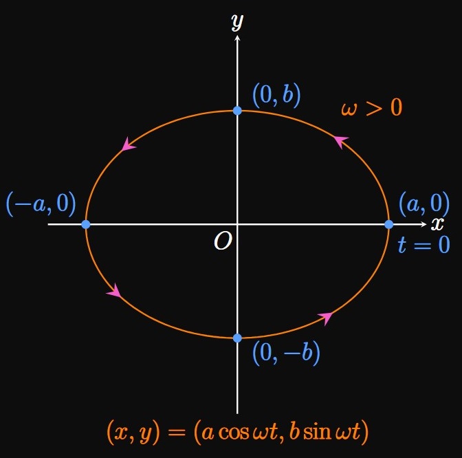
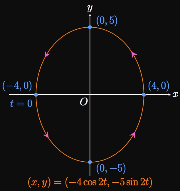
In Cartesian coordinates, the equation of an ellipse centered at the origin is \begin{equation} \frac{x^2}{a^2} + \frac{y^2}{b^2} = 1 \label{eq:cart-ellipse} \end{equation} for any real numbers \(a\) and \(b.\) To represent this curve using parametric equations, we want \(\eqrefer{eq:cart-ellipse}\) to match the form \(\cos^2 \omega t + \sin^2 \omega t = 1.\) We therefore let \[ \baat{2} \frac{x^2}{a^2} &= \cos^2 \omega t \implies x &&= \pm a \cos \omega t \nl \frac{y^2}{b^2} &= \sin^2 \omega t \implies y &&= \pm b \sin \omega t \pd \eaat \] Alternatively, we could compare \(\eqrefer{eq:cart-ellipse}\) to the form \(\sin^2 \omega t + \cos^2 \omega t = 1,\) from which we obtain \[ \baat{2} \frac{x^2}{a^2} &= \sin^2 \omega t \implies x &&= \pm a \sin \omega t \nl \frac{y^2}{b^2} &= \cos^2 \omega t \implies y &&= \pm b \cos \omega t \pd \eaat \] Thus, the ellipse of \(\eqref{eq:cart-ellipse}\) is parameterized by either \begin{flalign} && x &= \pm a \cos \omega t &&y = \pm b \sin \omega t \label{eq:para-ellipse-cos-sin} &\nl \laWord{or} && x &= \pm a \sin \omega t &&y = \pm b \cos \omega t \pd \label{eq:para-ellipse-sin-cos} \end{flalign} We parameterize an ellipse using \(\eqref{eq:para-ellipse-cos-sin}\) if the point \((x,y)\) is at the farthest left or farthest right of the ellipse when \(t = 0.\) By contrast, when \(t = 0\) \(\eqref{eq:para-ellipse-sin-cos}\) places \((x,y)\) at the top or bottom of the ellipse.

Planets' orbits are a major application of particle motion along ellipses. According to Kepler's First Law, planets' orbits around the Sun take the shape of an ellipse, with the Sun at one focus. Therefore, understanding parametric equations enables scientists to calculate the time in which a planet completes an orbit. Scientists can also estimate the date of an eclipse—a moment when one celestial body (for example, the Sun, Moon, or Earth) appears darkened as it passes through the shadow of another celestial body.

Let \(t\) be time in minutes; we therefore consider only \(t \geq 0.\) The ellipse's semi-minor axis has length \(4,\) and its semi-major axis has length \(5.\) From \(\eqref{eq:para-ellipse-cos-sin},\) parametric equations that model the starting point \((-4, 0)\) are \[x = -4 \cos \omega t \lspace y = \pm 5 \sin \omega t \pd\] One revolution occurs in \(\pi\) minutes, so \[\omega = \frac{2 \pi}{\pi} = 2 \pd\] Thus, our preliminary equations (without yet considering direction of motion) are \[x = -4 \cos 2t \lspace y = \pm 5 \sin 2t \pd\] The particle moves counterclockwise, so for small \(t \gt 0,\) \(x\) is increasing and \(y\) is decreasing. When \(t = 0,\) \(y = -5 \sin 2t\) is decreasing, as required. Thus, we choose the parametric equations \[\boxed{x = -4 \cos 2t} \and \boxed{y = -5 \sin 2t}\] (See Figure 9.)

The Cycloid

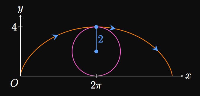
Imagine a circle rolling on the floor. As the circle rolls, a point on the circle's circumference traces out a shape called a cycloid. Animation 1 depicts a circle of radius \(1\) rolling along the ground, covering a total horizontal distance of \(4 \pi.\)

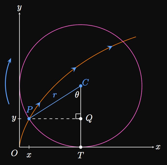
See Figure 10: To write parametric equations for the cycloid, we find the \(x\)- and \(y\)-coordinates of a point \(P\) on the circumference as functions of the parameter \(\theta,\) which is subtended by the line segments \(\segment{PC}\) and \(\segment{TC}.\) Before the circle begins rolling, \(\theta = 0\) and so point \(P\) is at the origin \(O.\) As the circle rolls, \(P\) rotates clockwise and traces out the arc length \(r \theta.\) So the horizontal distance the circle has rolled is \[\length{OT} = \arc{PT} = r \, \theta \pd\] We therefore see \[ \baat{3} x &= \length{OT} - \length{PQ} &&= r \theta - r \sin \theta &&= r(\theta - \sin \theta) \nl y &= \length{CT} - \length{CQ} &&= r - r \cos \theta &&= r(1 - \cos \theta) \pd \eaat \] Thus, parametric equations for a cycloid formed by a circle of radius \(r\) are \begin{equation} x = r(\theta - \sin \theta) \lspace y = r(1 - \cos \theta) \pd \label{eq:cycloid} \end{equation}

Observe that the circle is inscribed within one arch of the cycloid at the peak \((2\pi, 4)\) (Figure 11). The circle's radius is therefore \(2,\) so by \(\eqref{eq:cycloid}\) a set of parametric equations is \[\boxed{x = 2(\theta - \sin \theta)} \and \boxed{y = 2(1 - \cos \theta)}\]

Projectile Motion

When an object is hit upward, it follows a parabolic trajectory due to the influence of gravity. (We will verify that the trajectory is indeed parabolic.) The motion of a projectile can be modeled using an \(xy\)-plane where \(y\) is the projectile's height above the ground and \(x\) is its ground position. We will call \(y\) the vertical direction and \(x\) the horizontal direction. The line \(y = 0\) is conveniently chosen to be the ground. During projectile motion, \(x\) and \(y\) both vary with time, independent of each other. In other words, at any time \(t\) the projectile's height and ground position are changing separately. Using parametric equations is therefore useful because they enable us to consider the motion along each direction.

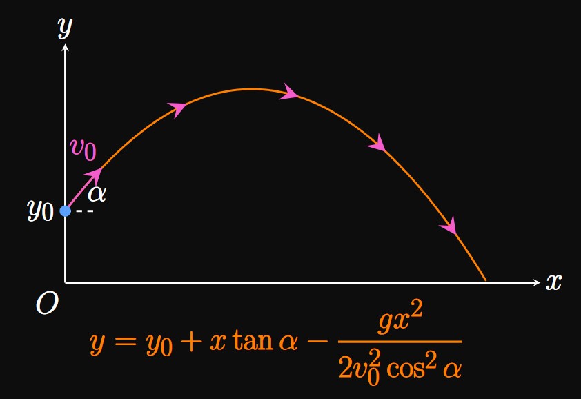
Suppose an object at point \(P,\) a height \(y_0\) above the ground, is thrown upward with initial velocity \(v_0\) at an angle \(\alpha\) above the ground (Figure 12). Observe that the initial velocity has two components: \(v_0 \cos \alpha\) (the initial velocity in the horizontal direction) and \(v_0 \sin \alpha\) (the initial velocity in the vertical direction). The acceleration due to gravity points straight down and has magnitude \(g,\) whose value is \(32 \undiv{ft}{sec}^2\) or \(9.8 \undiv{m}{sec}^2.\) In words, after every second the object's vertical velocity is decreasing by \(32 \undiv{ft}{sec}.\) We neglect air resistance and drag.

Horizontal \((x)\) Direction There is no acceleration in the \(x\)-direction because no forces act on the falling object in the horizontal direction. Consequently, the object's speed in the horizontal direction is constantly \(v_0 \cos \alpha\) until the object strikes the ground. If velocity is constant, then displacement is the product of velocity and time. Accordingly, at any time \(t\) the object's horizontal position is \[ x = v_0 (\cos \alpha) t \pd \]

Vertical \((y)\) Direction Let \(y\) be the object's height above the ground, and suppose \(y_0\) is the object's initial height. We pick the upward direction to be positive. In the vertical direction, the acceleration is uniformly \(-g\) (negative because it points downward) and the initial velocity is \(v_0 \sin \alpha\) (positive because it points upward). Using the methods of antidifferentiation and substituting initial conditions (from Section 4.1, in which we modeled solely the height of an object in free fall), we attain \[ y = y_0 + v_0 (\sin \alpha) t - \tfrac{1}{2} gt^2 \pd \]

Let \(t\) be time in seconds; we consider the ball's trajectory to be a parabola in the \(xy\)-plane (Figure 13).

1. The initial velocity is \(v_0 = 64 \undiv{ft}{sec},\) and the angle is \(\alpha = 30 \degree.\) Since the ball is kicked from the ground, its initial height is \(0.\) By \(\eqref{eq:projectile-motion},\) parametric equations for the ball's trajectory are \[ \baat{2} x &= 64 (\cos 30 \degree) t = \boxed{(32 \sqrt 3) t} \nl y &= 0 + 64(\sin 30 \degree) t - \tfrac{1}{2}(32)t^2 &&= \boxed{32 t - 16 t^2} \eaat \] for all \(t\) such that \(y \geq 0.\)

---

2. The ball reaches the ground when \(y = 0 \col\) \[32t - 16t^2 = 0 \implies t = 0 \cma t = 2 \pd\] So the ball hits the ground after \(\boxed{2}\) seconds. Thus, the parametric equations in part (a) are restricted by \(0 \leq t \leq 2.\)

---

3. Because the trajectory is parabolic, the ball reaches its maximum height \(H\) halfway before reaching the ground—that is, when \(t = 1.\) The maximum height is therefore \[y(1) = 32(1) - 16(1)^2 = \boxed{16 \un{ft}}\]

---

4. The total horizontal distance \(D\) traveled by the ball is given by \[x(2) = (32 \sqrt 3)(2) \approx 110.851 \un{ft}\pd\] This value is less than \(200 \un{ft},\) so the ball does not reach the goal. Accordingly, the player does not score.

We seek to model the trajectory's shape without using time \(t,\) so we eliminate the parameter in \begin{equation} x = v_0 (\cos \alpha) t \lspace y = y_0 + v_0 (\sin \alpha) t - \tfrac{1}{2} gt^2 \pd \eqlabel{eq:projectile-motion} \end{equation} The simplest method is as follows: Solving for \(t\) in the first parametric equation gives \[t = \frac{x}{v_0 \cos \alpha} \pd\] Substituting this expression into the second parametric equation, we attain \[ y = y_0 + v_0 (\sin \alpha) \par{\frac{x}{v_0 \cos \alpha}} - \tfrac{1}{2} g \par{\frac{x}{v_0 \cos \alpha}}^2 \pd \] Simplifying gives \[ \boxed{y = y_0 + x \tan \alpha - \frac{gx^2}{2 v_0^2 \cos^2 \alpha}} \] Because \(y\) is a second-degree polynomial in \(x\) (note that all other quantities are constants), we have proved that the trajectory of an object undergoing free fall is a parabola (Figure 14).