8.1: Slope Fields and Euler's Method

It turns out that a ball in free fall produces a parabolic trajectory, whereas a population of animals grows exponentially. As we will learn later in this chapter, we can predict these systems' behaviors by analyzing their differential equations. Differential equations are extremely powerful tools in science, economics, and ecology. We discuss the following topics:

• Defining a Differential Equation
• Slope Fields
• Euler's Method

Defining a Differential Equation

A differential equation relates a function to its independent variable and derivatives. Generally, a differential equation in \(y\) and \(x\) is some equation that includes \(x,\) \(y,\) and the derivatives of \(y.\) In an algebraic equation we solve for some unknown value, such as solving for \(a\) in the equation \(3a - 6 = 0.\) Yet the solution to a differential equation is a function. In Section 4.1 we discussed the simplest type of differential equation: \[\deriv{y}{x} = f(x) \cma\] whose general solution is the function \(y = \int f(x) \di x + C.\) An \(\bf n\)th-order differential equation includes an \(n\)th-order derivative as its highest-order derivative. An example of a second-order differential equation is \[\derivOrder{y}{x}{2} + \deriv{y}{x} + 5y = 0\] because the highest-order derivative has order \(2.\) In this chapter we focus primarily on first-order differential equations, which relate the rate of change of \(y\)—that is, \(\textderiv{y}{x}\)—to \(x\) and \(y.\) As an example, the first-order differential equation \[\deriv{y}{x} = x + y\] asserts that the rate at which \(y\) changes with \(x\) equals the sum of \(x\) and \(y.\)

Particular Solutions Recall, from Section 4.1, that we often combine a differential equation with an initial condition. This pair is called an initial value problem. In particular, we seek some function \(f(x)\) that solves a differential equation while satisfying \(f \par{x_0} = y_0.\) Then \(f(x)\) is called a particular solution to that differential equation, and \(f \par{x_0} = y_0\) is an initial condition.

Slope Fields

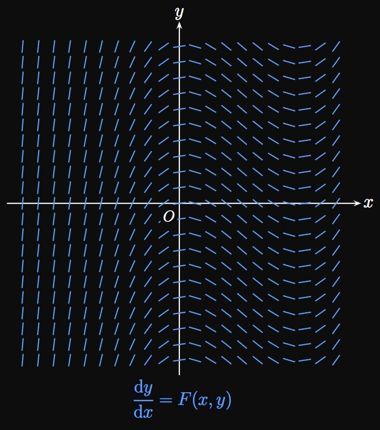
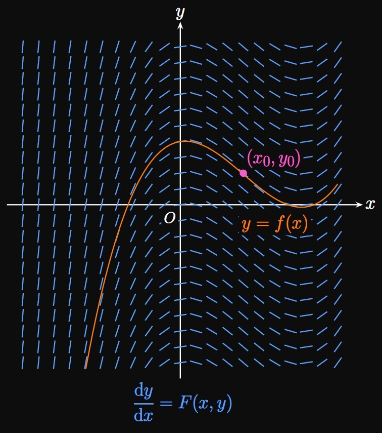
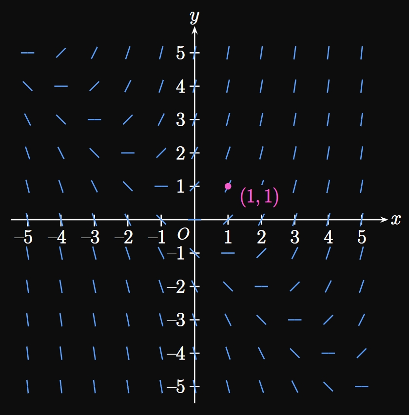
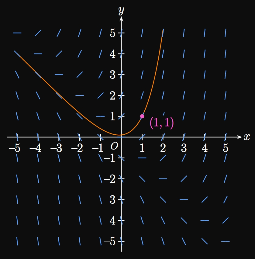
Most differential equations are very difficult or even impossible to solve analytically. Consider the first-order differential equation \[\deriv{y}{x} = F(x, y) \cma\] where \(F(x, y)\) is some expression containing \(x\) and \(y.\) Regardless of whether this differential equation can be solved, we can better understand this model by drawing short line segments of slope \(F(x, y)\) at several points \((x, y).\) The result is a slope field (or direction field), which provides the blueprint for a solution curve. Figure 1A shows the slope field for some differential equation \(\textderiv{y}{x} = F(x, y).\) Each line segment indicates the direction in which a solution curve travels at \((x, y).\) A particular solution curve is a graph that follows a slope field and passes through some point \(\par{x_0, y_0};\) for example, Figure 1B shows the particular solution curve \(y = f(x)\) that satisfies the initial condition \(y_0 = f(x_0).\)

At each of points \(A,\) \(B,\) and \(C,\) we compute the slope \(\textderiv{y}{x} = x^2 - 2y.\) The slope at \(A(0, 1)\) is \[(0)^2 - 2(1) = -2 \pd\] So in the \(xy\)-plane, we draw a line segment of slope \(-2\) at the point \((0, 1).\) Likewise, the slope at \(B(2, -1)\) is \[(2)^2 - 2(-1) = 6 \pd\] We therefore sketch a line segment of slope \(6\) at the point \((2, -1).\) Lastly, the slope at \(C(2, 2)\) is \[(2)^2 - 2(2) = 0 \pd\] Hence, we draw a horizontal line segment at the point \((2, 2).\) The slope field for these three points is shown in Figure 2.

Which choice could be the differential equation for the slope field in Figure 3?

1. \(\ds \deriv{y}{x} = x\)
2. \(\ds \deriv{y}{x} = y\)
3. \(\ds \deriv{y}{x} = x + y\)
4. \(\ds \deriv{y}{x} = xy\)

At any \((x, y),\) the slope is \(\textderiv{y}{x} = x - y.\) To construct a slope field, we evaluate \(\textderiv{y}{x}\) at several points of \((x, y).\) The following observations help us sketch the field:

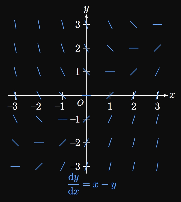
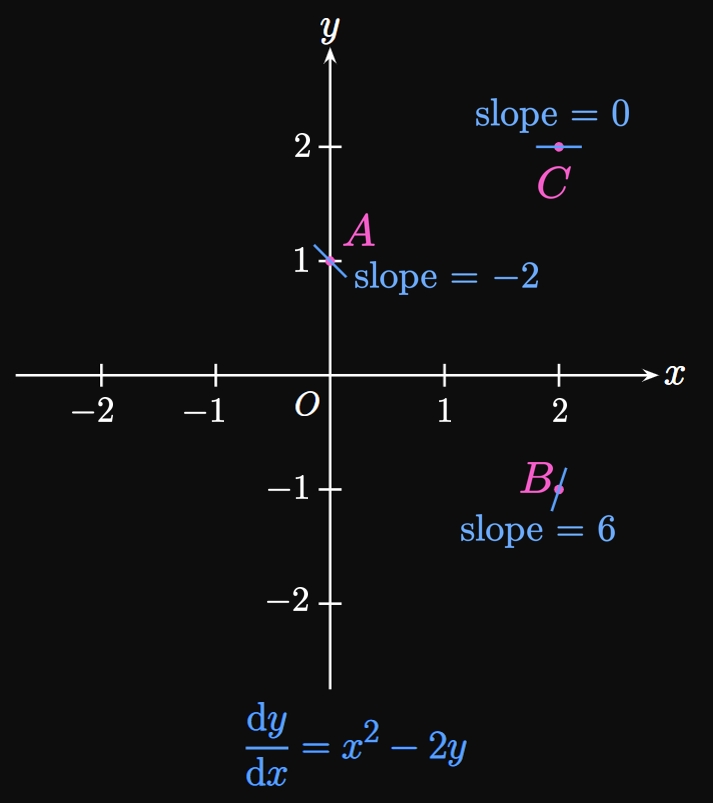
• When \(x = y,\) we see \(x - y = 0.\) Thus, the slope is \(0\) at the points \((1, 1),\) \((2, 2),\) \((3, 3)\) and \((-1, -1),\) \((-2, -2),\) \((-3, -3).\) We therefore draw short horizontal line segments at these points.
• When \(x\) is negative and \(y\) is positive, \(\textderiv{y}{x} = x - y \lt 0.\) So the slopes are negative in the second quadrant.
• In the fourth quadrant, the slopes are positive because \(x\) is positive and \(y\) is negative.
• When \(x\) is bigger than \(y,\) the slope is positive. Conversely, when \(x\) is smaller than \(y,\) the slopes are negative.

We therefore attain the slope field in Figure 4.

For the slope field in Figure 5, sketch the particular solution curve that passes through the point \((1, 1).\)

Starting at the point \((1, 1),\) we follow the direction of the nearby line segments. The slope is positive at \((1, 1),\) so from this point we trace the curve upward and rightward—roughly parallel to the nearby line segments. Conversely, to the left of \((1, 1),\) we extend the curve downward and leftward (according to the direction of the nearby slopes), until it attains a relative minimum at \(x = 0.\) Afterward, we sketch the curve leftward and upward to match the slopes of the line segments. The solution curve should be parallel to the nearby line segments. (See Figure 6.)

Euler's Method

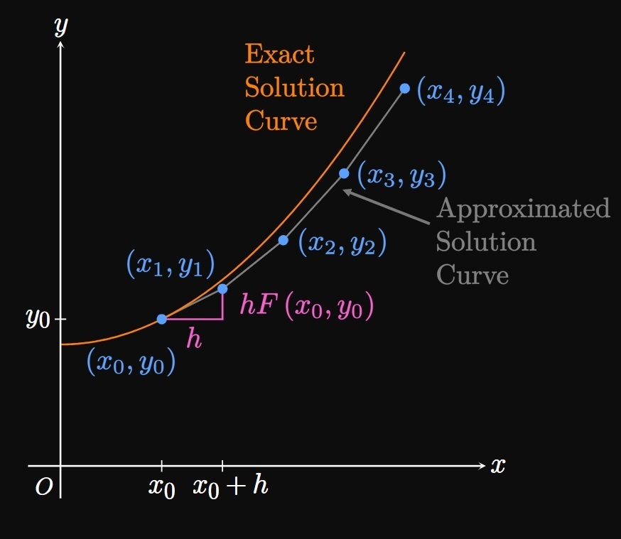
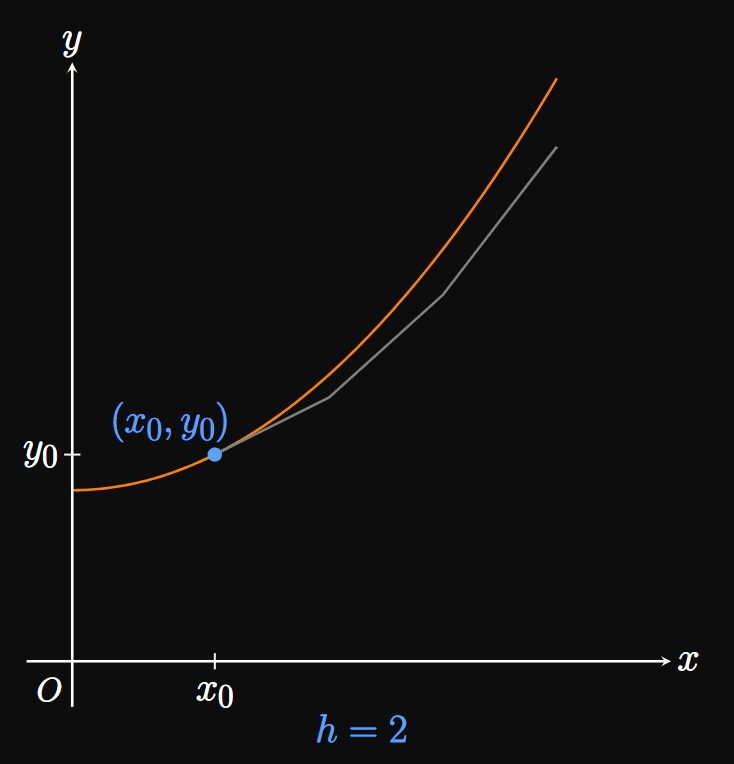
Most differential equations have no analytical solutions; we must therefore use a method to approximate particular solutions. Given a differential equation \[\deriv{y}{x} = F(x, y) \cma\] Euler's Method enables us to estimate a particular solution with the initial condition \(y \par{x_0} = y_0\) by using a series of linear approximations. We approximate points on the solution curve at equally spaced numbers \(x_0,\) \(x_1 = x_0 + h,\) \(x_2 = x_1 + h, \dots.\) We call \(h\) the step size, the amount by which we increment \(x\) as we take more and more approximation points. In Figure 7 a solution curve is approximated by the points \(\par{x_0, y_0},\) \(\par{x_1, y_1},\) \(\par{x_2, y_2},\) \(\par{x_3, y_3},\) and \(\par{x_4, y_4}.\) The slope at \(\par{x_0, y_0}\) is \(F \par{x_0, y_0},\) so we have \[y_1 = y_0 + hF\par{x_0, y_0} \pd\] Likewise, we observe that \[y_2 = y_1 + h F \par{x_1, y_1} \pd\] In general, the horizontal distance between any points \(\par{x_{n - 1}, y_{n - 1}}\) and \(\par{x_n, y_n}\) is the step size \(h;\) the vertical distance is \(hF\par{x_{n - 1}, y_{n - 1}}.\) Mathematically, \begin{equation} y_n = y_{n - 1} + hF\par{x_{n - 1}, y_{n - 1}} \pd \label{eq:euler-method} \end{equation} In words, we attain each subsequent approximation for \(y\) by adding on the slope \(F\par{x_{n - 1}, y_{n - 1}}\) multiplied by the step size \(h.\) Why is this useful? Remember that the slope \(F(x, y)\) is known, while the exact solution curve is unknown. Euler's Method therefore enables us to approximate a solution curve by using its rate of change \(F.\) Methodically, we begin at the point \(\par{x_0, y_0}\) and proceed in the direction of the slope field. After \(x\) is incremented by a distance \(h,\) we take the slope at the new location and traverse in that direction. We repeat this process until \(x\) is some desired number. Doing so gives us several points that we can plot to approximate a solution curve. Observe that the first step in Euler's Method is a linearization for \(y_1\) (see Section 2.8). Decreasing the step size \(h\) allows us to sample more points, so the approximated solution curve better fits the exact solution curve. (See Animation 1.) This method lets computers output accurate solutions to many differential equations whose solutions are difficult to obtain. Even a spreadsheet is sufficient to use Euler's Method, and many computer-algebra systems produce slope fields for us—the beauty of technology in the modern world.