7.3: Consumer Surplus and Producer Surplus

In a market, producers and consumers are both driven by benefit. In economics, we need a way to measure how much each party benefits from the sale of an item at some price level. We do so through the following topics:

• Consumer Surplus
• Producer Surplus

Consumer Surplus

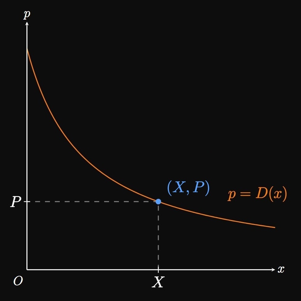
Demand Curves Recall, from Section 3.7, that an inverse relationship exists between price and the number of goods sold (by the Law of Demand). The demand function \(p = D(x)\) models the price per unit that a firm can charge to sell \(x\) units. Figure 1 shows a typical demand curve: We plot \(x\) on the horizontal axis, and we plot the good's price p on the vertical axis. The function \(D(x)\) is the price at which \(x\) units of a commodity are demanded. To sell \(X\) units of a good, a company must sell the product at \(P = D(X)\) dollars.

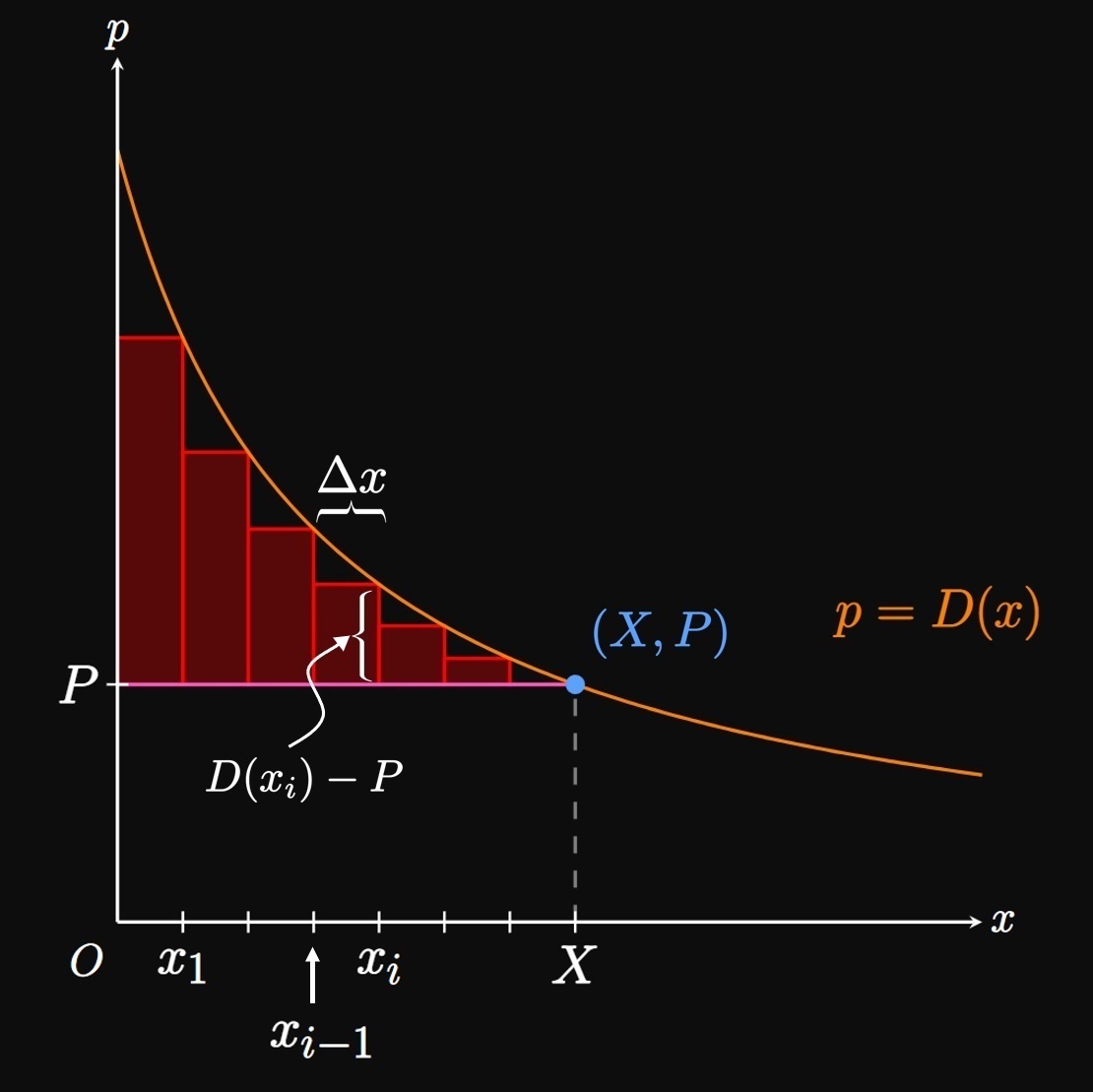
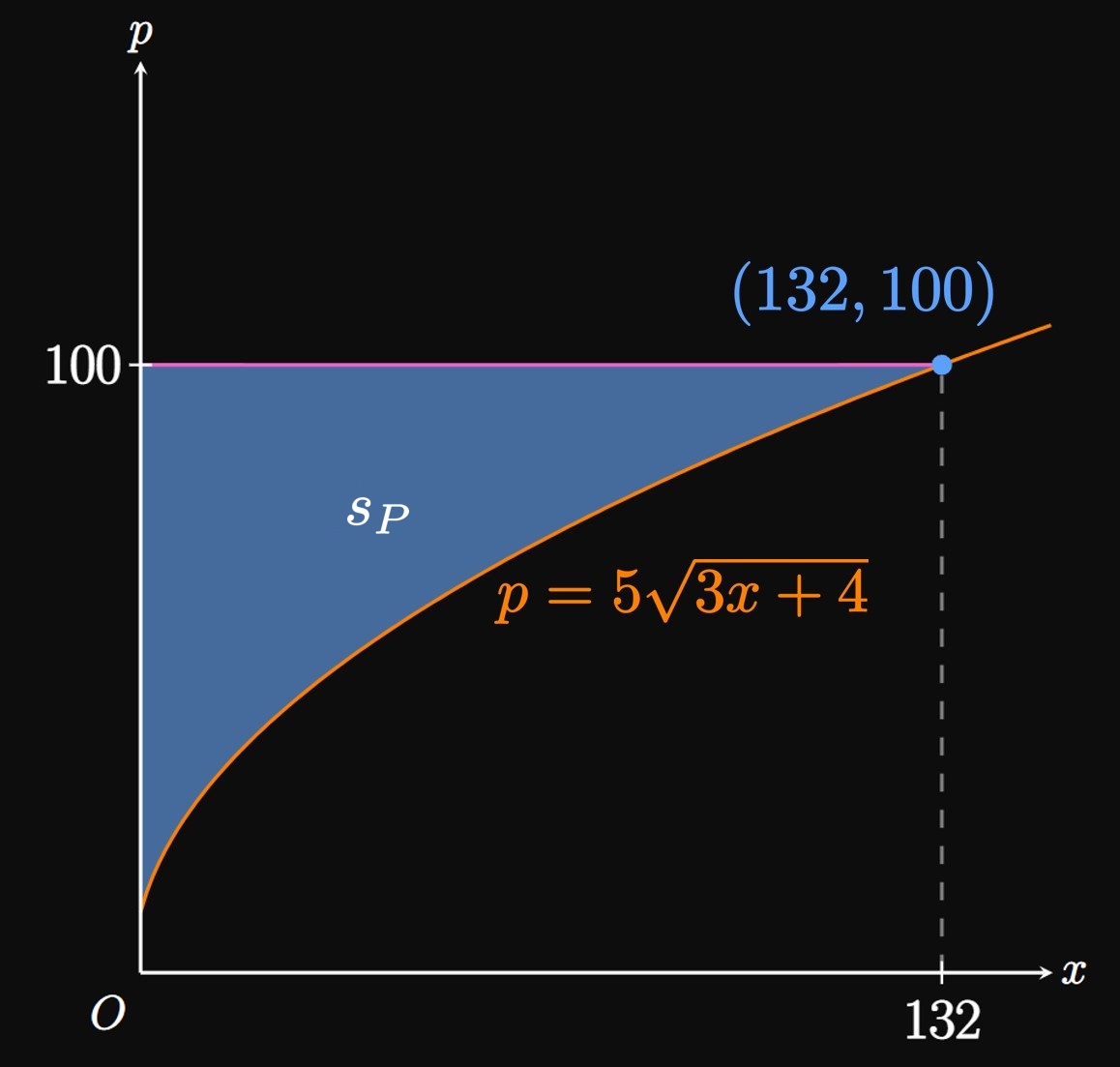
But some consumers are willing to pay more for a product; these shoppers are therefore pleased to pay less. Consumer surplus measures this level of benefit among all customers. To calculate consumer surplus, we divide the interval \([0, X]\) into \(n\) subintervals of endpoints \(0 = x_0,\) \(x_1, \dots,\) \(x_{n - 1}, x_n = X\) and equal width \(\Delta x = X/n.\) Imagine that each subinterval represents a group of \(\Delta x\) items sold. In a general subinterval \([x_{i - 1}, x_i],\) we inscribe a rectangle at the right endpoint \(x_i^* = x_i.\) Observe that \(x_{i - 1}\) units are sold if the price is \(D(x_{i - 1})\) dollars. Yet to increase sales to \(x_i\) units, the price must be lowered to \(D(x_i)\) dollars. Each consumer who was willing to pay \(D(x_i)\) dollars (instead of \(P\) dollars) saved \(D(x_i) - P\) dollars. Hence, the total savings in the subinterval \([x_{i - 1}, x_i]\) is approximately \[(\text{savings per unit}) \, (\text{number of units}) = \parbr{D(x_i) - P} \Delta x \pd\] This product is the area of an approximating rectangle in Figure 2. Adding the savings across all \(n\) subintervals, we attain the following estimate for consumer surplus: \[s_C = \sum_{i = 1}^n \parbr{D(x_i) - P} \Delta x \pd\] This expression is a Riemann sum for the function \(D(x) - P.\) As we increase \(n,\) we sample more groups of units sold. Letting \(n \to \infty,\) \(\Delta x \to 0\) and so we attain the definite integral \begin{equation} s_C = \int_0^X \parbr{D(x) - P} \di x \pd \label{eq:s-c} \end{equation} Accordingly, the consumer surplus \(s_C\) is the area bounded under the demand curve \(p = D(x)\) and above the line \(p = P.\) (See Figure 3.)

The consumer surplus \(s_C\) is the area of the region bounded above by the demand curve and below by the line \(p = 800.\) To find the quantity demanded at this price, we solve \(D(X) = 800 \col\) \[1200 - \frac{X^2}{100} = 800 \implies X^2 = 40\cmaNum000 \implies X = 200 \pd\] We ignore the solution \(X = -200\) because the quantity demanded cannot be negative. (See Figure 4.) Thus, following \(\eqref{eq:s-c},\) we find the consumer surplus to be \[ \ba s_C &= \int_0^{200} \parbr{\par{1200 - \frac{x^2}{100}} - 800} \di x \nl &= \int_0^{200} \par{400 - \frac{x^2}{100}} \di x \nl &= \par{400x - \frac{x^3}{300}} \intEval_0^{200} \nl &= \boxed{\frac{160\cmaNum000}{3}} \approx \$53\cmaNum333.33 \pd \ea \]

Producer Surplus

Supply Functions A supply function \(p = S(x)\) gives the price \(p\) at which \(x\) units of a good are supplied. Whereas the Law of Demand models an inverse relationship between price and quantity demanded, the Law of Supply asserts that a direct relationship exists between price and quantity supplied. For example, few companies are interested in manufacturing and selling a phone for just \(\$100.\) But if the phone's market price is \($900,\) then many more companies are attracted to the market, meaning the quantity of phones supplied increases. Figure 5 shows a typical supply curve, in which \(X\) units of a good are supplied if the good is sold at \(P\) dollars.

Similar to the idea in Consumer Surplus, a company may be willing to sell goods for cheaper than the market price \(P.\) Producer surplus can be interpreted as the benefit to a firm by selling units at a higher price \(P.\) We split the interval \([0, X]\) into \(n\) equally sized subintervals of size \(\Delta x = X/n.\) A firm is willing to sell \(x_{i - 1}\) units at a price of \(S(x_{i - 1})\) dollars, but will only sell \(\Delta x\) more products if the price is raised to \(S(x_{i})\) dollars. By selling the product at \(P\) dollars instead of \(S(x_{i})\) dollars, the firm gains \(P - S(x_i)\) per unit. So the firm's gain from selling \(\Delta x\) units is approximately \[(\text{gain per unit}) \, (\text{number of units}) = \parbr{P - S(x_i)} \Delta x \pd\] Let's add the gain over the \(n\) equally sized subintervals in \([0, X];\) doing so, the producer surplus is approximated by \[s_P = \sum_{i = 1}^n \parbr{P - S(x_i)} \Delta x \pd\] If we let \(n \to \infty,\) then this sum becomes the definite integral \begin{equation} s_P = \int_0^X \parbr{P - S(x)} \di x \pd \label{eq:p-surplus} \end{equation} Hence, producer surplus is the area bounded below by the supply curve and above by the line \(p = P\) (Figure 6).

The artist supplies enough skateboards such that \(S(X) = 100.\) (If she supplied more than \(X\) skateboards, then she would be losing money.) Solving this equation, we see \[5 \sqrt{3X + 4} = 100 \implies 3X + 4 = 400 \implies X = 132 \pd\] The producer surplus is the area bounded above by the line \(p = 100\) and below by the supply curve from \(x = 0\) to \(x = 132.\) (See Figure 7.) Following \(\eqref{eq:p-surplus},\) we find the producer surplus to be \[s_P = \int_0^{132} \par{100 - 5 \sqrt{3x + 4}} \di x \pd\] Substituting \(u = 3x + 4,\) we have \(\dd u = 3 \di x.\) When \(x = 0,\) \(u = 4;\) when \(x = 132,\) \(u = 400.\) So the integral becomes \[ \ba s_P &= \tfrac{1}{3} \int_4^{400} \par{100 - 5\sqrt u \,} \di u \nl &= \tfrac{1}{3} \par{100 u - \tfrac{10}{3} u^{3/2}} \intEval_4^{400} \nl &= \boxed{\$4320} \ea \]