2.1: Defining a Derivative
In Chapter 1 we studied limits and continuity, but how are they used in defining advanced concepts in calculus? In this section we learn the fundamentals of differential calculus—the study of rates of change. We discuss the following topics:
- Definition of a Derivative
- Differentiability
- Derivative Properties
- Higher-Order Derivatives
- Position, Velocity, and Acceleration
Definition of a Derivative
A fundamental part of calculus is calculating a function's slope at a point. This slope represents the function's rate of change at an exact moment. Calculating slopes allows us to delve into the realm of instantaneous rates; we can find how rapidly a population is increasing or how quickly a deflating balloon's radius is shrinking—fundamental skills in the study of differential calculus. The question is, what method do we use to find a function's slope?
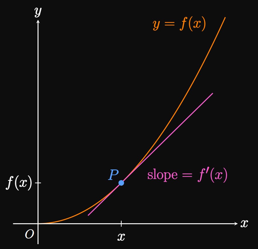
Geometry with Tangents The first half of the answer is to construct a tangent line to the function's graph. This line's slope matches the slope of the function. Figure 1 shows the graph of a function \(f\) and the tangent line to \(f\) at point \(P(x, f(x)),\) which "just touches" the graph of \(f\) at \(P.\) The slope of \(f\) at \(P\)—and, accordingly, of the tangent line at \(P\)—has slope \(f'(x),\) called a derivative. The derivative \(f'(x)\) measures the rate of change of \(f\) at \(x \col\) If \(f\) increases steeply at \(x,\) then \(f'(x)\)—the slope of \(f(x)\)—is a large positive number. In contrast, if \(f\) is decreasing at \(x,\) then \(f'(x)\) is negative because the slope of \(f(x)\) is negative. We formally define a tangent line using the derivative, as follows.
The tangent line doesn't necessarily touch the graph only once, because the line could strike the graph at any point farther away. The second part of our question is set: what is our procedure to compute the slope of the tangent line?
Calculating a Derivative
The second half of our answer is to construct a line that collapses into
the tangent line, and calculate the slope as the line transforms into a tangent line.
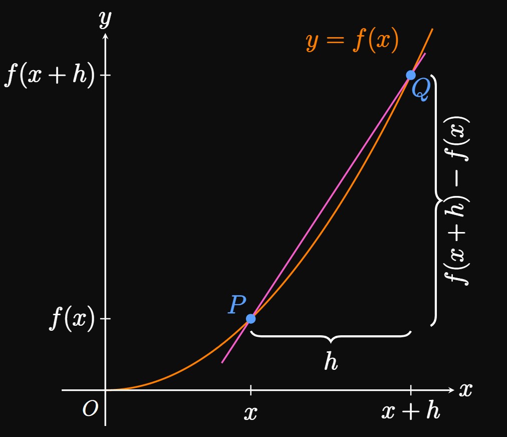
As in Figure 2,
we construct a secant line that
intersects \(f\) at points \(P\) and \(Q,\)
both on the graph of \(f.\)
If the horizontal difference between \(P\) and \(Q\) is \(h,\)
then the vertical difference is \(f(x + h) - f(x).\)
Therefore, the slope of the secant line is
\[m_{PQ} = \frac{\Delta y}{\Delta x} = \frac{f(x + h) - f(x)}{h} \pd\]
We call \(m_{PQ}\) a difference quotient because it's a ratio of two differences.
If we move \(Q\) along the graph of \(f\) to be closer to \(P\)—that is, if \(h\)
shrinks—then the secant line better resembles the tangent line to \(P.\)
If \(h\) is made infinitely close to \(0,\)
then the secant line becomes the tangent line, as in Animation 1.
Therefore, we find the slope of the tangent line by taking the limit of \(m_{PQ}\) as \(h \to 0;\) namely,
\begin{equation}
f'(x) = \lim_{h \to 0} \frac{f(x + h) - f(x)}{h} \pd \label{eq:lim-defn}
\end{equation}
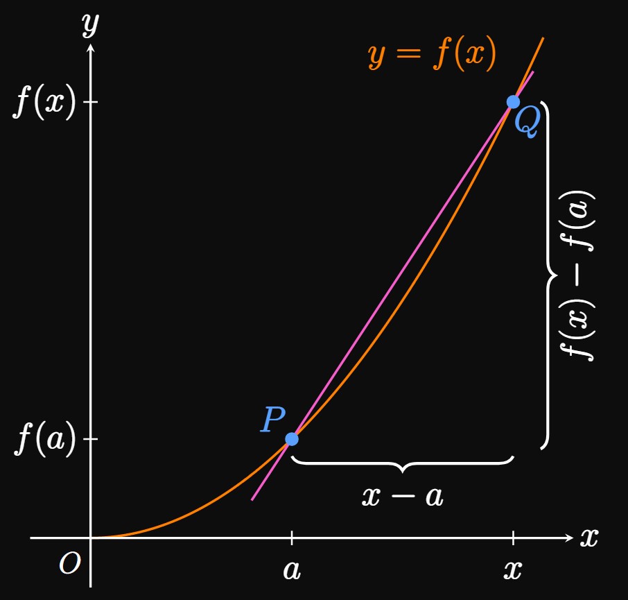
There is another definition of the derivative. If we draw a secant line that intersects the graph of \(f\) at points \(P(a, f(a))\) and \(Q(x, f(x)),\) then the secant line's slope is \[m_{PQ} = \frac{f(x) - f(a)}{x - a} \pd\] (See Figure 3.) Then as \(x\) is made closer to \(a,\) the secant line begins to collapse into the tangent line to \(f\) at \(P.\) We then get \begin{equation} f'(a) = \lim_{x \to a} \frac{f(x) - f(a)}{x - a} \pd \label{eq:lim-defn-point} \end{equation} We use \(\eqrefer{eq:lim-defn-point}\) to find a derivative of \(f\) at a specific point \((a, f(a)).\) In contrast, \(\eqrefer{eq:lim-defn}\) gives the derivative of \(f\) as a function of \(x,\) that is, the slope of \(f\) as a function of \(x.\) To find a derivative of a function at a point, we can use either difference quotient in \(\eqref{eq:lim-defn}\) or \(\eqref{eq:lim-defn-point}.\) Sometimes one form is easier to use than the other.
We pronounce \(\textDeriv{y}{x}\) as "\(\dd y\) by \(\dd x\)" or simply "\(\dd y,\) \(\dd x.\)" Using Leibniz notation, we can also write \[\deriv{y}{x} = \deriv{}{x} (y) \pd\] The expression \(\textDeriv{}{x}\) is an operator, whereas \(\textDeriv{y}{x}\) is a quantity. An analogy is as follows: \(\textDeriv{}{x}\) is a verb, and \(\textDeriv{y}{x}\) is a noun. To denote the derivative of \(y = f(x)\) at a point \(x = a,\) in Leibniz notation we write \(\textDeriv{f}{x}|_{x = a}\) or \(\textDeriv{y}{x}|_{x = a},\) and in prime notation we write \(f'(a)\) or \(y'(a).\) Taking a derivative is called differentiation.
We seek the derivative at a specific point. Hence, we can use either \(\eqref{eq:lim-defn}\) or \(\eqref{eq:lim-defn-point},\) with \(x = 2.\) If we use \(\eqref{eq:lim-defn-point},\) then \(f(x) = 1/x\) and \(f(2) = 1/2,\) and \[f'(2) = \lim_{x \to 2} \frac{1}{x - 2} \left(\frac{1}{x} - \frac{1}{2}\right) \pd\] We cannot perform direct substitution by immediately substituting \(x = 2,\) because this limit is of the indeterminate form \(\indZero.\) Our strategy is then to combine the fractions using a common denominator and attempt to cancel a common factor. (See Section 1.2 for a review of finding indeterminate limits.) Doing so gives \[ \ba f'(2) &= \lim_{x \to 2} \frac{1}{x - 2} \left(\frac{2 - x}{2x}\right) \nl &= \lim_{x \to 2} \frac{1}{x - 2} \left(\frac{-(x - 2)}{2x}\right) \nl &= \lim_{x \to 2} \frac{-1}{2x} \nl &= \boxed{-\frac{1}{4}} \ea \]
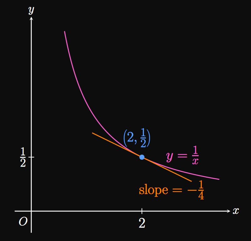
We interpret this value as follows: The tangent line to the graph of \(y = 1/x\) at \(x = 2\) has a slope of \(-1/4.\) (See Figure 4.)
If we chose to use \(\eqref{eq:lim-defn}\) to find \(f'(2),\) then our limit would have been \[f'(2) = \lim_{h \to 0} \frac{1}{h} \left(\frac{1}{2 + h} - \frac{1}{2}\right) \pd\] You may verify that this limit also equals \(-1/4,\) matching the answer we obtained using \(\eqref{eq:lim-defn-point}.\)
- \(\ds \deriv{}{x}(3x + 2)\)
- \(\ds \deriv{}{x} \par{x^2}\)
- \(\ds \deriv{}{x} \par{\sqrt x \,}\)
- Using \(\eqref{eq:lim-defn},\) we have \(f(x) = 3x + 2\) and \(f(x + h) = 3(x + h) + 2.\) Thus, \[ \ba \deriv{}{x} (3x + 2) &= \lim_{h \to 0} \frac{f(x + h) - f(x)}{h} \nl &= \lim_{h \to 0} \frac{[3(x + h) + 2] - [3x + 2]}{h} \pd \ea \] Simplification of the limit gives \[ \ba \deriv{}{x}[3x + 2] &= \lim_{h \to 0} \frac{3h}{h} \nl &= \lim_{h \to 0} 3 \nl &= \boxed{3} \ea \]
- Using \(\eqref{eq:lim-defn},\) with \(f(x) = x^2\) and \(f(x + h) = (x + h)^2,\) we obtain \[\deriv{}{x} \par{x^2} = \lim_{h \to 0} \frac{(x + h)^2 - x^2}{h} \pd\] We cannot immediately substitute \(h = 0\) in the difference quotient, as we get the indeterminate form \(\indZero.\) Instead, we expand \((x + h)^2\) and cancel terms. This strategy gives \[ \ba \deriv{}{x} \par{x^2} &= \lim_{h \to 0} \frac{x^2 + 2xh + h^2 - x^2}{h} \nl &= \lim_{h \to 0} \frac{2xh + h^2}{h} \nl &= \lim_{h \to 0} (2x + h) \nl &= \boxed{2x} \ea \]
- We use \(\eqref{eq:lim-defn}\) with \(f(x) = \sqrt x\) and \(f(x + h) = \sqrt{x + h}.\) The derivative is then \[\deriv{}{x} \par{\sqrt x \,} = \lim_{h \to 0} \frac{\sqrt{x + h} - \sqrt x}{h} \pd\] This limit is in the indeterminate form \(\indZero.\) Since the fraction contains radicals, our strategy is to multiply the numerator and denominator by the conjugate of the numerator, namely, \(\sqrt{x + h} + \sqrt x.\) Doing so, we find \[ \ba \deriv{}{x} \par{\sqrt x \,} &= \lim_{h \to 0} \frac{\sqrt{x + h} - \sqrt x}{h} \cdot \frac{\sqrt{x + h} + \sqrt x}{\sqrt{x + h} + \sqrt x} \nl &= \lim_{h \to 0} \frac{(x + h) - x}{h \par{\sqrt{x + h} + \sqrt x}} \nl &= \lim_{h \to 0} \frac{h}{h \par{\sqrt{x + h} + \sqrt x}} \nl &= \lim_{h \to 0} \frac{1}{\sqrt{x + h} + \sqrt x} \nl &= \frac{1}{\sqrt{x + 0} + \sqrt x} \nl &= \boxed{\frac{1}{2 \sqrt x}} \ea \]
Differentiability
If \(f'(a)\) is defined, then we say function \(f\) is differentiable at \(a.\) We call a function differentiable if its derivative is defined at each point in its domain. Differentiability implies continuity: if \(f\) is differentiable at \(a,\) then \(f\) is continuous at \(a.\) But the converse statement is not necessarily true—a function can be continuous but not differentiable at a point. All differentiable functions are continuous, but not all continuous functions are differentiable.
A derivative may fail to exist for several reasons: If \(f\) is discontinuous at \(a,\) then \(f'(a)\) doesn't exist because differentiability requires continuity. If \(f\) is continuous at \(a,\) then \(f'(a)\) fails to exist
- if at \(x = a\) the left-hand derivative and right-hand derivative of \(f\) don't match; or
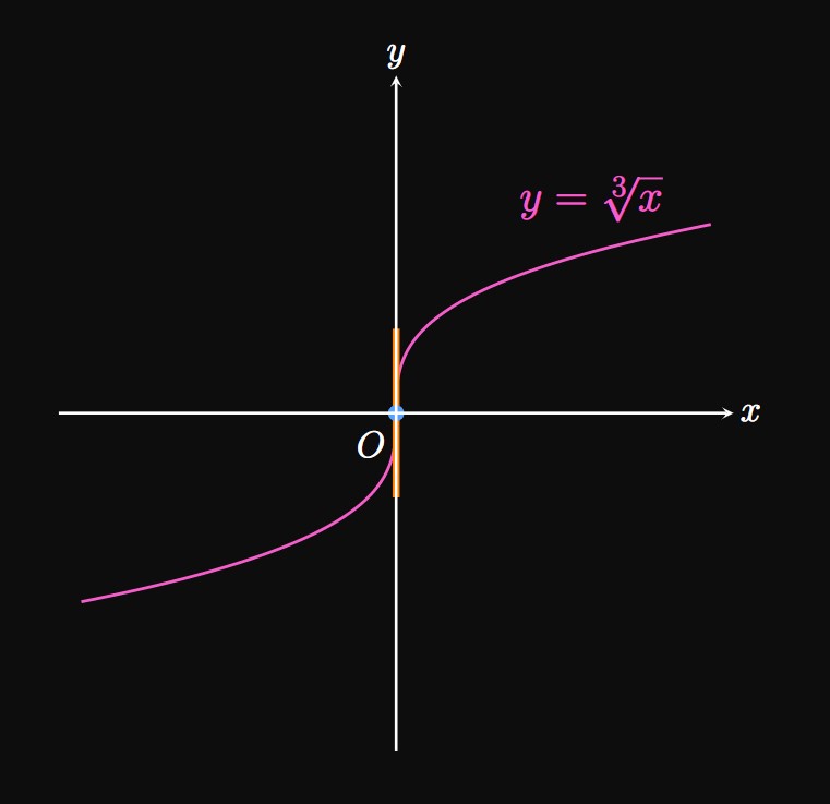
- if \(f\) has a vertical tangent line at \(x = a.\)
- \(f(x)\) is discontinuous at \(x = a.\)
- The one-sided derivatives of \(f(x)\) at \(x = a\) are not equivalent.
- \(f(x)\) has a vertical tangent at \(x = a.\)
- \(g'(-4)\)
- \(g'(-3)\)
- \(g'(0)\)
- \(g'(2)\)
- \(g'(3)\)
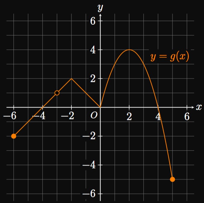
- At \(x = -4\) the slope of \(g\) is \(1.\) Therefore, \(g'(-4) = \boxed 1.\)
- Because \(g(-3)\) is undefined, \(g\) is discontinuous at \(x = -3.\) Hence, \(g'(-3)\) is undefined.
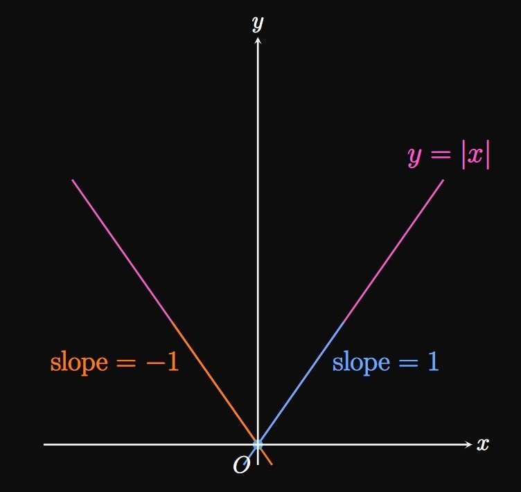
- Function \(g\) has a sharp turn at \(x = 0.\) Specifically, at \(x = 0\) the left-hand derivative of \(g\) is \(-1\) and the right-hand derivative is a positive number. Since these values are not equivalent, \(g'(0)\) is undefined.
- The tangent line to \(g\) at \(x = 2\) is horizontal and therefore has slope \(0.\) Thus, \(g'(2) = \boxed 0.\)
- If we draw a tangent line to \(g\) at \(x = 3,\) then we see this line has slope \(-2.\) Hence, \(g'(3) = \boxed{-2}.\)
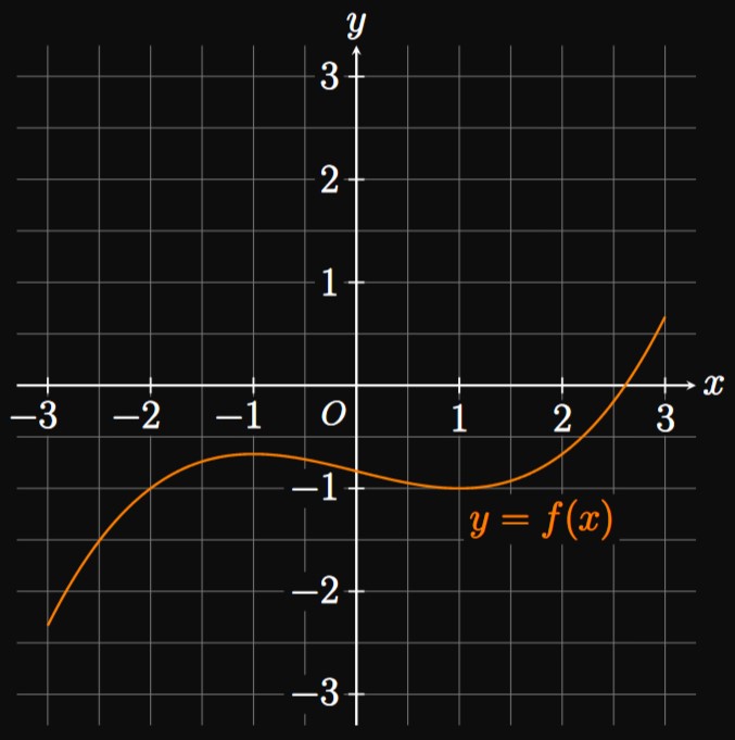
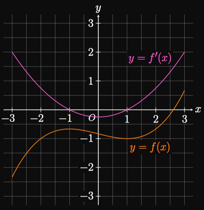
- \(f(x)\) has horizontal tangent lines when \(x = -1\) and \(x = 1.\) Since these lines each have slope \(0,\) \(f'(-1) = f'(1) = 0.\)
- \(f(x)\) is increasing over \(-3 \leq x \leq -1\) and \(1 \leq x \leq 3.\) Thus, \(f'\)—the slope of \(f\)—is positive for \(-3 \lt x \lt -1\) and \(1 \lt x \lt 3.\)
- \(f(x)\) is decreasing over \(-1 \leq x \leq 1.\) Accordingly, \(f'\) is negative for \(-1 \lt x \lt 1.\)
Derivative Properties
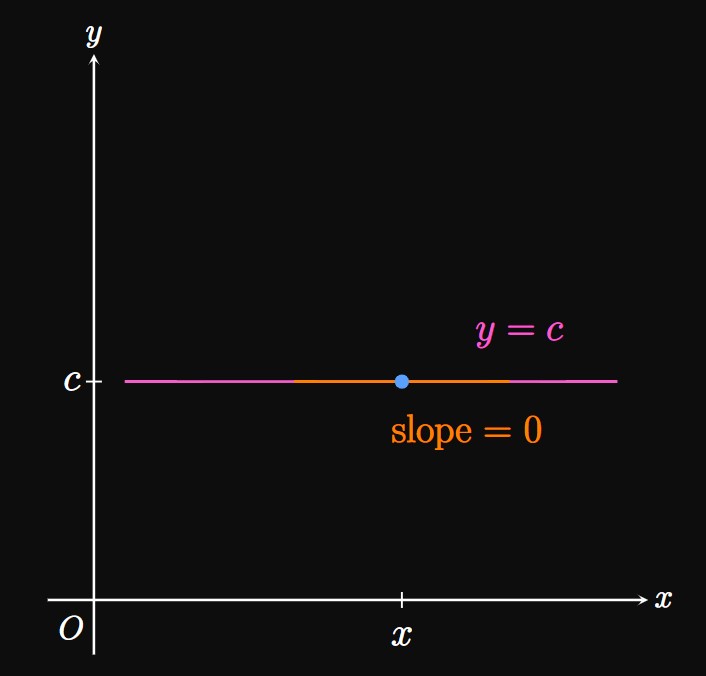
The derivative of any constant \(c\) is \(0.\) We affirm this result geometrically because the graph of \(y = c\) is flat and therefore has a slope of \(0\) at all points (Figure 10). The proof of this fact is as follows.
PROOF Let \(f(x) = c,\) where \(c\) is a constant. We want to prove that \(f'(x) = 0.\) Using \(\eqrefer{eq:lim-defn},\) both \(f(x)\) and \(f(x + h)\) equal \(c\) because \(f(x)\) does not depend on \(x.\) Thus, we have \begin{align*} f'(x) &= \lim_{h \to 0} \frac{f(x + h) - f(x)}{h} \nl &= \lim_{h \to 0} \frac{c - c}{h} \nl &= \lim_{h \to 0} \frac{0}{h} \nl &= 0 \pd \end{align*} \[\qedproof\] Note that the limit \(\lim_{h \to 0} (0/h)\) is not in the indeterminate form \(\indZero,\) since the numerator is fixed at \(0.\)
In addition, the derivative of a function multiplied by a constant is the constant multiplied by the derivative. Also, the derivative of a sum is the sum of derivatives, and the derivative of a difference is the difference of derivatives. These properties are summarized below.
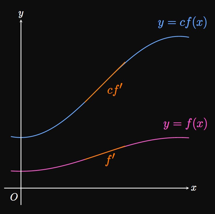
PROOF OF CONSTANT MULTIPLE RULE The limit definition of \(\textderiv{}{x} [cf(x)]\) is \[\deriv{}{x} [c f(x)] = \lim_{h \to 0} \frac{[cf(x + h)] - [cf(x)]}{h} \pd\] Factoring out \(c\) shows \[ \ba \deriv{}{x} [c f(x)] &= c \lim_{h \to 0} \frac{f(x + h) - f(x)}{h} \nl &= c f'(x) \pd \ea \] \[\qedproof\] A visual interpretation of this property is shown in Figure 11, in which the slope of \(y = c f(x)\) is \(c\) times the slope of \(y = f(x)\) at some \(x.\)
PROOF OF SUM AND DIFFERENCE RULES The limit definition of \((f + g)'(x)\) is \[(f + g)'(x) = \lim_{h \to 0} \frac{[f(x + h) + g(x + h)] - [f(x) + g(x)]}{h} \pd\] We regroup the terms in the numerator and split the limit by the Sum Law for Limits. (See Section 1.2 for a review of limit properties.) We find \[ \ba (f + g)'(x) &= \lim_{h \to 0} \frac{[f(x + h) - f(x)] + [g(x + h) - g(x)]}{h} \nl &= \lim_{h \to 0} \frac{f(x + h) - f(x)}{h} + \lim_{h \to 0} \frac{g(x + h) - g(x)}{h} \nl &= f'(x) + g'(x) \pd \ea \] Similarly, the limit definition of \((f - g)'(x)\) is \[(f - g)'(x) = \lim_{h \to 0} \frac{[f(x + h) - g(x + h)] - [f(x) - g(x)]}{h} \pd\] Rearranging and splitting the limit, using the Difference Law for Limits, give \[ \ba (f - g)'(x) &= \lim_{h \to 0} \frac{[f(x + h) - f(x)] - [g(x + h) - g(x)]}{h} \nl &= \lim_{h \to 0} \frac{f(x + h) - f(x)}{h} - \lim_{h \to 0} \frac{g(x + h) - g(x)}{h} \nl &= f'(x) - g'(x) \pd \ea \] Hence, \((f + g)'(x) = f'(x) + g'(x)\) and \((f - g)'(x) = f'(x) - g'(x).\) \[\qedproof\]
- \(\ds \deriv{}{x} [f(x) + g(x)]_{x = 2}\)
- \(\ds \deriv{}{x} [f(x) - g(x)]_{x = -3}\)
- \(\ds \deriv{}{x} [2f(x)]_{x = 1}\)
- \(\ds \deriv{}{x} [2f(x) - 3g(x)]_{x = 3}\)
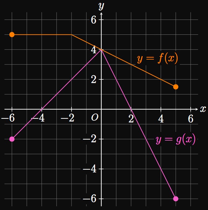
- By the Sum Rule for Derivatives, the derivative of a sum is the sum of derivatives. Thus, \[ \deriv{}{x} [f(x) + g(x)]_{x = 2} = f'(2) + g'(2) \pd \] In Figure 12, at \(x = 2\) the slope of \(f\) is \(-1/2\) and the slope of \(g\) is \(-2.\) Accordingly, \(f'(2) = -1/2\) and \(g'(2) = -2,\) and \[\deriv{}{x} [f(x) + g(x)]_{x = 2} = -\tfrac{1}{2} - 2 = \boxed{-\tfrac{5}{2}}\]
- The Difference Rule states that the derivative of a difference is the difference of derivatives: \[\deriv{}{x} [f(x) - g(x)]_{x = -3} = f'(-3) - g'(-3) \pd\] At \(x = -3,\) the slope of \(f\) is \(0\) and the slope of \(g\) is \(1.\) Thus, \(f'(-3) = 0\) and \(g'(-3) = 1,\) so \[\deriv{}{x} [f(x) - g(x)]_{x = -3} = 0 - 1 = \boxed{-1}\]
- By the Constant Multiple Rule, we can take out the constant in the derivative: \[\deriv{}{x} [2f(x)]_{x = 1} = 2 f'(1) \pd\] At \(x = 1\) the slope of \(f\) is \(-1/2.\) We therefore have \[\deriv{}{x} [2f(x)]_{x = 1} = 2 \left(-\tfrac{1}{2}\right) = \boxed{-1}\]
- Combining the Constant Multiple Rule and Difference Rule gives \[ \ba \deriv{}{x} [2f(x) - 3g(x)]_{x = 3} &= \deriv{}{x} [2f(x)]_{x = 3} - \deriv{}{x}[3g(x)]_{x = 3} \nl &= 2f'(3) - 3g'(3) \pd \ea \] At \(x = 3,\) the slope of \(f\) is \(-1/2\) and the slope of \(g\) is \(-2.\) Hence, \(f'(3) = -1/2\) and \(g'(3) = -2;\) therefore, \[\deriv{}{x} [2f(x) - 3g(x)]_{x = 3} = 2 \left(-\tfrac{1}{2}\right) - 3(-2) = \boxed{5}\]
Function \(g\) is differentiable at \(2\) if \(g\) is continuous at \(2\) and the one-sided derivatives of \(g\) at \(2\) are equal. We assert that \(g\) is continuous at \(2\) if \(\lim_{x \to 2} g(x) = g(2).\) (See Section 1.4 to review continuity.) The left-hand limit of \(g\) at \(2\) is \[\lim_{x \to 2^-} g(x) = 4(2) - 1 = 7 \pd\] The right-hand limit of \(g\) at \(2\) is \[\lim_{x \to 2^+} g(x) = (2)^2 + 3 = 7 \pd\] Since these values are the same, \(\lim_{x \to 2} g(x)\) exists and equals \(7,\) which is \(g(2).\) Hence, \(g\) is continuous at \(x = 2.\)
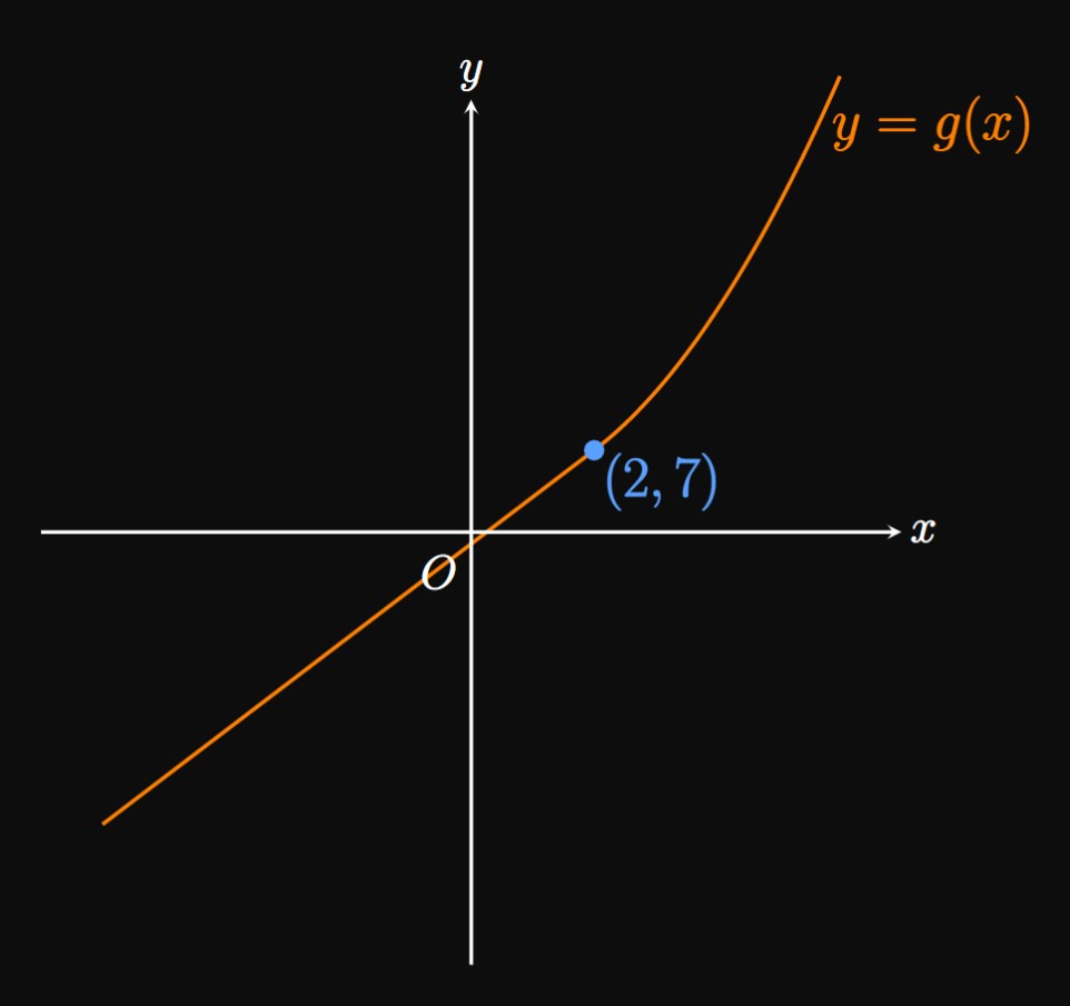
The one-sided derivatives of \(g\) at \(2\) must equal each other. The left-hand derivative of \(g(x)\) at \(x = 2\) is \(\textDeriv{}{x} \, [4x - 1]_{x = 2},\) which by \(\eqref{eq:lim-defn}\) is \[ \ba \lim_{h \to 0^-} \frac{[4(2 + h) - 1] - [4(2) - 1]}{h} &= \lim_{h \to 0^-} \frac{4h}{h} \nl &= 4 \pd \ea \] Likewise, at \(x = 2\) the right-hand derivative of \(g\) is \(\textDeriv{}{x} \, [x^2 + 3]_{x = 2},\) which is \[ \ba \lim_{h \to 0^+} \frac{[(2 + h)^2 + 3] - [(2)^2 + 3]}{h} &= \lim_{h \to 0^+} \frac{4h + h^2}{h} \nl &= \lim_{h \to 0^+} (4 + h) \nl &= 4 \pd \ea \] Since both one-sided derivatives of \(g\) at \(2\) are equivalent, \(g'(2)\) exists. Hence, \(g(x)\) is differentiable at \(x = 2.\) The graph of \(y = g(x)\) is shown in Figure 13.
Higher-Order Derivatives
Physical scenarios often exhibit higher-order derivatives. We denote the second derivative of \(y\) with respect to \(x\) as \(\textDerivOrder{y}{x}{2};\) that is, \[\derivOrder{y}{x}{2} = \deriv{}{x} \left(\deriv{y}{x} \right) \pd\] The \(n\)th derivative of \(y\) is \(\textDeriv{^n y}{x^n}.\) (Be careful of the superscript position.) In prime notation the second derivative of \(y = f(x)\) with respect to \(x\) is \(f''(x)\) or \(y''(x),\) and the \(n\)th derivative is \(f^{(n)}(x)\) or \(y^{(n)}(x).\) [Do not write \(f^{n}(x).\)] The key to taking higher-order derivatives is to differentiate incrementally: Differentiate once to determine the first derivative, and then differentiate the resulting expression to find the second derivative. Repeat this process as many times as necessary.
Another notation for the derivative is the dot notation, named after Isaac Newton. This form solely denotes a derivative with respect to time; for example, the derivative of \(y\) with respect to time is \(\dot y.\) Likewise, the second derivative of \(y\) with respect to time is \(\ddot y.\) This notation is most commonly used in physics.
Position, Velocity, and Acceleration
We define an object's position to be how far the object is from a reference point. If \(s(t)\) gives an object's position at time \(t,\) then the object's velocity \(v(t)\) is the rate at which the object's position changes with respect to time—that is, \begin{equation} v(t) = \deriv{s}{t} \pd \label{eq:v(t)-deriv} \end{equation} Velocity is an object's speed in a certain direction; we choose an axis orientation such that one direction is positive and the other is negative. For example, if we select east to be the positive direction, then a car driving east has a positive velocity, while a car driving west has a negative velocity. \(\eqrefer{eq:v(t)-deriv}\) gives the rate at which an object's position changes at an instant. Accordingly, we can call \(v(t)\) the object's instantaneous velocity. The rate at which velocity changes with respect to time is acceleration, \(a(t)\)—namely, \begin{equation} a(t) = \deriv{v}{t} = \derivOrder{s}{t}{2} \pd \label{eq:a(t)-deriv} \end{equation} Suppose that you're driving a car and the positive direction of motion is the direction you're facing. The car's velocity increases when you step on the gas pedal, so the car is accelerating. In contrast, pressing the brake pedal decreases the car's velocity, thus decelerating the car.
Units Since velocity is the rate at which position is changing with time, the unit of velocity is the position unit per time unit. Similarly, acceleration is the rate at which velocity changes with time, so the unit of acceleration is the velocity unit per time unit. For example, if position is measured in meters and time is measured in seconds, then the velocity's unit is meters per second. Likewise, acceleration's unit is meters per second per second, or meters per second squared.
By \(\eqrefer{eq:v(t)-deriv}\) the particle's velocity function is the derivative of position with respect to time; namely, \(v(t) = s'(t).\) We seek the derivative of position as a function, so we use \(\eqref{eq:lim-defn}\) to get \[ \ba v(t) &= s'(t) \nl &= \lim_{h \to 0} \frac{[3(t + h)^2 + 2] - [3t^2 + 2]}{h} \nl &= \lim_{h \to 0} \frac{6ht + 3h^2}{h} \nl &= \lim_{h \to 0} (6t + h) \nl &= 6t \pd \ea \] Hence, the particle's velocity function is \(v(t) = 6t.\)
The particle's acceleration function is, by \(\eqref{eq:a(t)-deriv},\) the derivative of the velocity function. Hence, \(a(t) = v'(t) = \textDeriv{}{t} \, [6t].\) We obtain \[ \ba a(t) &= v'(t) \nl &= \lim_{h \to 0} \frac{6(t + h) - 6t}{h} \nl &= \lim_{h \to 0} \frac{6h}{h} \nl &= \lim_{h \to 0} 6 \nl &= 6 \pd \ea \] The particle's acceleration function is therefore \(a(t) = 6.\)
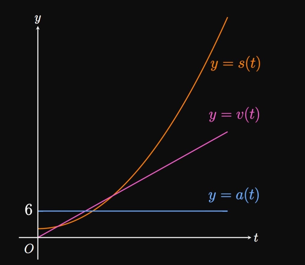
The graphs of \(s(t),\) \(v(t),\) and \(a(t)\) are shown by Figure 15. Their domains are each \(t \geqslant 0\) since time can't be negative. When \(t = 2,\) the particle's velocity is \(v(2) = 12\) inches per minute and the particle's acceleration is \(a(2) = 6\) inches per minute squared.
Definition of a Derivative The derivative of a function \(f\) at \(x\) measures the slope of \(f\) at \(x.\) We denote the derivative either using prime notation \((f')\) or Leibniz notation \((\textDeriv{f}{x}).\) In Leibniz notation \(\textDeriv{}{x}\) is an operator, whereas \(\textDeriv{f}{x}\) is a quantity. Dot notation \((\dot f)\) represents the derivative of a function with respect to time and is commonly seen in physics.
Derivative as a Function The process of calculating the derivative of \(f\) at point \(P(x, f(x))\) is as follows: Construct a secant line that passes through point \(P\) and another point \(Q(x + h, f(x + h))\) on the graph of \(f.\) By taking \(h \to 0,\) the secant line becomes the tangent line, whose slope is \begin{equation} f'(x) = \lim_{h \to 0} \frac{f(x + h) - f(x)}{h} \pd \eqlabel{eq:lim-defn} \end{equation} If the limit exists, then \(\eqref{eq:lim-defn}\) gives the derivative of \(f\) as a function of \(x;\) we call \(f'\) the derivative function of \(f.\)
Derivative at a Point The derivative of the function \(f(x)\) at the point \(x = a\) is \begin{equation} f'(a) = \lim_{x \to a} \frac{f(x) - f(a)}{x - a} \eqlabel{eq:lim-defn-point} \end{equation} if the limit exists. This form is an alternate definition of the derivative.
Differentiability If \(f'(a)\) is defined, then function \(f\) is differentiable at \(a.\) A function is called differentiable if its derivative is defined at each point in its domain. Differentiability requires continuity. All differentiable functions are continuous, but not all continuous functions are differentiable. A derivative \(f'(a)\) fails to exist due to any of the following reasons:
- \(f(x)\) is discontinuous at \(x = a.\)
- The one-sided derivatives of \(f(x)\) at \(x = a\) are not equivalent.
- \(f(x)\) has a vertical tangent at \(x = a.\)
Derivative Properties Let \(f\) and \(g\) be differentiable functions, and let \(c\) be a constant. Then the following properties hold: \[ \baat{2} & \deriv{}{x} (c) = 0 \cma &&\comment{\text{Constant Rule}} \nl & \deriv{}{x} [c f(x)] = c f'(x) \cma &&\comment{\text{Constant Multiple Rule}} \nl & \deriv{}{x} [f(x) + g(x)] = f'(x) + g'(x) \cma &&\comment{\text{Sum Rule}} \nl & \deriv{}{x} [f(x) - g(x)] = f'(x) - g'(x) \pd &&\comment{\text{Difference Rule}} \eaat \]
Higher-Order Derivatives Using prime notation, the second derivative of \(y = f(x)\) is \(f''(x)\) or \(y''(x).\) The \(n\)th derivative is \(f^{(n)}(x)\) or \(y^{(n)}(x).\) Do not write \(f^{n}(x).\) In Leibniz notation, we have \[\derivOrder{y}{x}{2} = \deriv{}{x} \left(\deriv{y}{x} \right) \pd\]
Position, Velocity, and Acceleration An object's position measures how far it is from an arbitrary reference point. The velocity is the rate at which the object's position changes with time, and the acceleration is the rate at which the object's velocity changes with time. If \(s(t)\) is position, \(v(t)\) is velocity, and \(a(t)\) is acceleration—all functions of time, \(t\)—then \[v(t) = \deriv{s}{t} \and a(t) = \deriv{v}{t} = \derivOrder{s}{t}{2} \pd \]